ECE 486 Control Systems
Lecture 6
Second Order System (Continued)
Last time we learned how to visualize system dynamics with block diagrams, especially all-integrator diagrams and basic system interconnections. We also began our discussion of prototype second order transfer function. We shall continue our investigation.
Recall from last time, the unit step response of a prototype underdamped second order transfer function \[ H(s) = \frac{\omega^2_n}{s^2 + 2\zeta\omega_n s + \omega^2_n} = \frac{\omega^2_n}{(s+\sigma)^2 + \omega^2_d} \] can be obtained as \[ y(t) = 1-e^{-\sigma t} \left(\cos(\omega_d t) + \frac{\sigma}{\omega_d}\sin(\omega_d t)\right), \] where \(\sigma = \zeta \omega_n\) and \(\omega_d = \omega_n \sqrt{1-\zeta^2}\) is the damped natural frequency.
We will see that the damping ratio \(\zeta\) and natural frequency \(\omega_n\) determine certain important features of the transient part of the above step response. We will also learn how to pick \(\zeta\) and \(\omega_n\) in order to shape these features according to given specifications.
Transient Response Specifications
Rise Time
We will start by taking a look at first order step response though.
\begin{align*} H(s) = \frac{a}{s+a}, \text{ with } a > 0. \end{align*}It has a stable pole \(s = -a\) since \(a\) is positive. By FVT, its DC gain is \(1\). (How?)
We can write down its unit step response as
\begin{align*} y(t) &= \LL^{-1} \{Y(s)\} \\ &= \LL^{-1} \left\{ H(s)\frac{1}{s} \right\} \\ &= \LL^{-1} \left\{ \frac{a}{s(s+a)} \right\} \\ &= \LL^{-1} \left\{ \frac{1}{s} - \frac{1}{s+a} \right\} \\ &= 1(t) - e^{-at}. \end{align*}We define rise time as the time it takes to get from 10% to 90% of steady-state value (of a step response). Rise time is denoted \(t_r\). Figure 1 shows the rise time of step response of a first order transfer function.
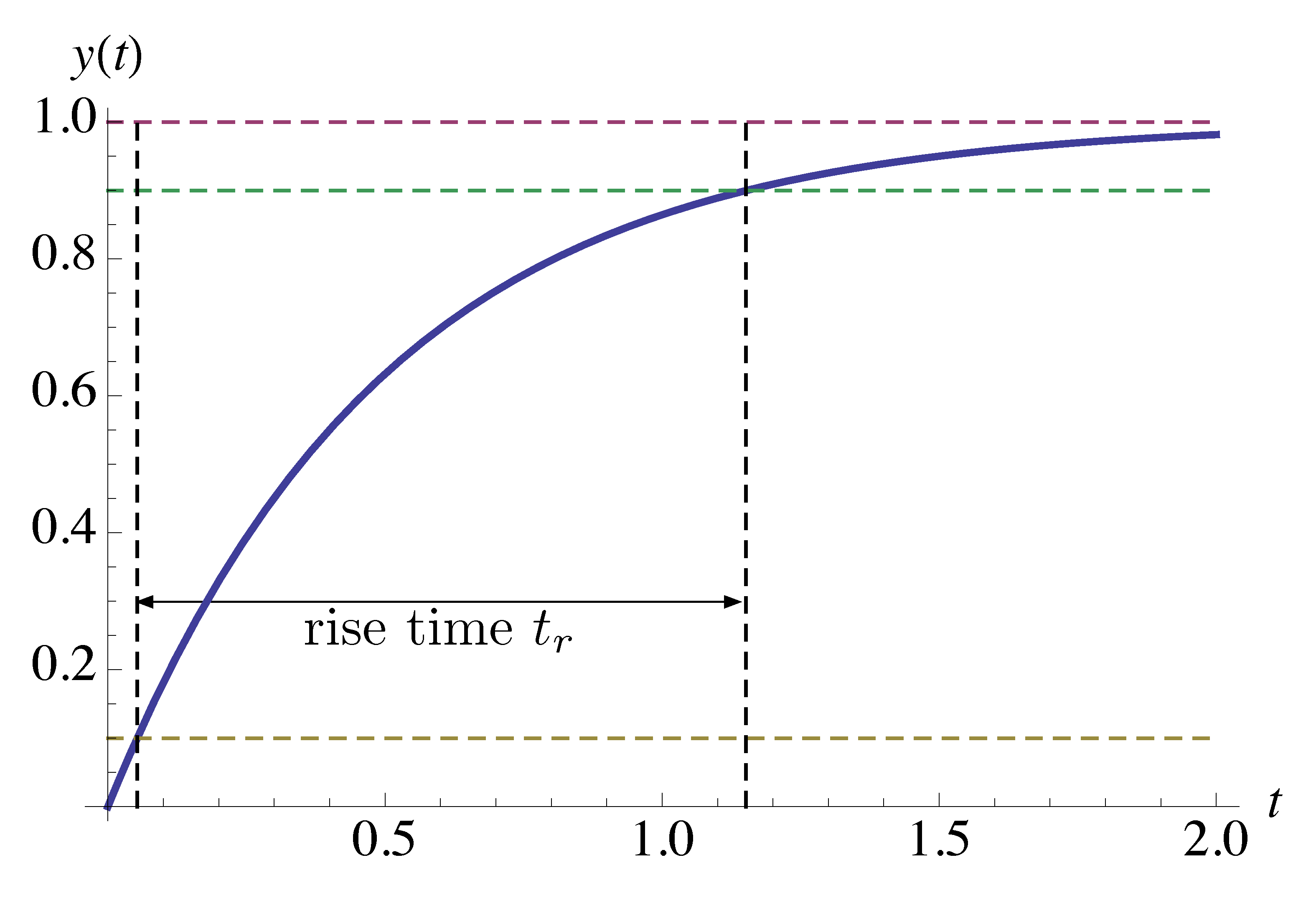
Figure 1: Rise time of a first order system
To compute \(t_r\) analytically in this example for step response \(y(t) = 1(t) - e^{-at}\), we follow the above definition: denote \(t_{0.1}\) and \(t_{0.9}\) as the time instances when it reaches 10% and 90% of its steady-state value respectively (for the first time), then
\begin{align*} & 1-e^{-at_{0.1}} = 0.1, \qquad e^{-at_{0.1}}=0.9, \qquad t_{0.1} = - \frac{\ln 0.9}{a}; \\ & 1-e^{-at_{0.9}} = 0.9, \qquad e^{-at_{0.9}}=0.1, \qquad t_{0.9} = - \frac{\ln 0.1}{a}. \\ &t_r = t_{0.9} - t_{0.1} = \frac{\ln 0.9 - \ln 0.1}{a} = \frac{\ln 9}{a} \approx \frac{2.2}{a}. \end{align*}Overshoot and Settling Time
Now let’s consider the more interesting case of a second order step response. When underdamped,
\begin{align*} H(s) &= \frac{\omega^2_n}{s^2 + 2\zeta\omega_n s + \omega^2_n} = \frac{\omega^2_n}{(s+\sigma)^2 + \omega^2_d}, \end{align*}where \(\sigma = \zeta \omega_n\), \(\omega_d = \omega_n \sqrt{1-\zeta^2}\) with \(\zeta < 1\).
We can graph the step response \(y(t) = 1-e^{-\sigma t} \left(\cos(\omega_d t) + \dfrac{\sigma}{\omega_d}\sin(\omega_d t)\right)\) as shown in Figure 2.
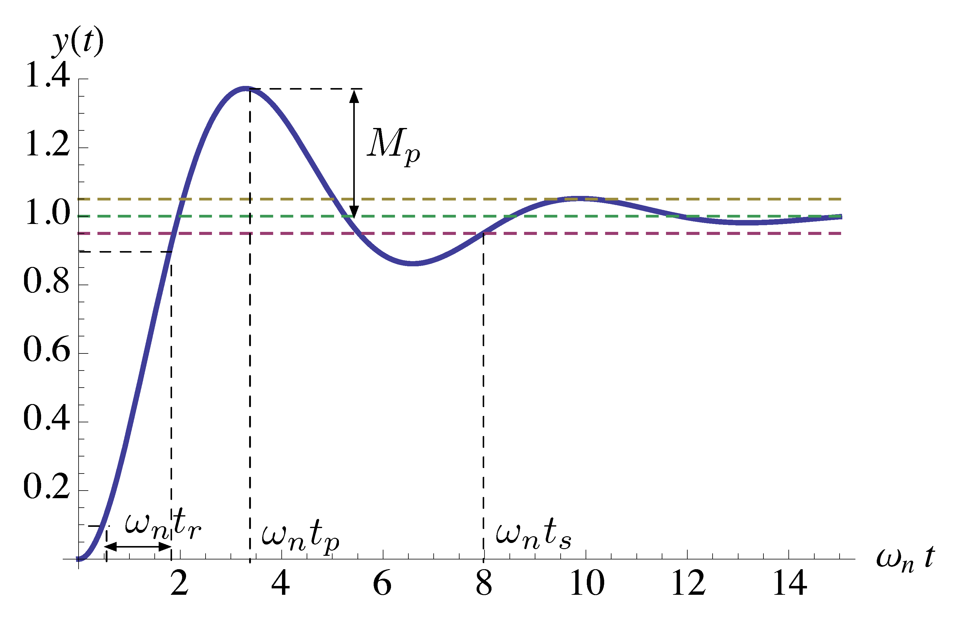
Figure 2: Rise time of a second order system (underdamped)
In addition to rise time, we also introduce two more specs: overshoot and settling time,
- Rise time \(t_r\): time to get from \(0.1 y(\infty)\) to \(0.9 y(\infty)\)
- Overshoot \(M_p\) and peak time \(t_p\) (note \(M_p\) could a percentage overshoot)
- Settling time \(t_s\): the first time for transients to decay to within a
specified small percentage of \(y(\infty)\) and stay in that range. We will
usually worry about 5% settling time; the default threshold for
stepinfo()inMatlabis 2%.
In general, the desired situation is to have fast rising, quickly settled step responses with low overshoot,
- \(t_r\), small
- \(M_p\), small
- \(t_p\), small
- \(t_s\), small
but it is impossible because of the trade-off that decreasing \(t_r\) leads to increased \(M_p\).
Formulas for Time Domain Specifications
Rise Time
Rise time \(t_r\) is hard to calculate analytically in general, but empirically, on the normalized time scale \(t \to \omega_n t\), rise times are approximately the same as
\[ w_n t_r \approx 1.8. \qquad \text{(exact when $\zeta = 0.5$)} \]
So, we will work with \(t_r \approx \dfrac{1.8}{\omega_n}\). It is a good approximation when \(\zeta \approx 0.5\).
Overshoot and Peak Time
In Figure 2, peak time \(t_p\) is the first time \(t > 0\) when \(y'(t) = 0\). By
\begin{align*} y(t) &= 1-e^{-\sigma t} \left(\cos(\omega_d t) + \dfrac{\sigma}{\omega_d}\sin(\omega_d t)\right) \\ y'(t) &= \left(\frac{\sigma^2}{\omega_d} + \omega_d\right) e^{-\sigma t}\sin(\omega_d t) = 0 \text{ when } \omega_d t = 0,\pi,2\pi, \ldots, \end{align*}we get \(t_p = \dfrac{\pi}{\omega_d}\).
To find overshoot \(M_p\), plug this value into \(y(t)\),
\begin{align*} M_p &= y(t_p) -1 \\ &= - e^{-\frac{\sigma\pi}{\omega_d}} \left(\cos\left(\omega_d\frac{\pi}{\omega_d}\right) + \frac{\sigma}{\omega_d}\sin\left(\omega_d \frac{\pi}{\omega_d}\right) \right) \\ &= - \exp\left(-\frac{\sigma\pi}{\omega_d}\right) (-1 + 0)\\ &= \exp\left( - \frac{\pi\zeta}{\sqrt{1-\zeta^2}}\right). \end{align*}The formula for \(M_p\) is exact.
Settling Time
The settling time is the last moment the step response enters the (5%) error strip and never leaves from that point on, \[ t_s = \min \left\{ t > 0: \, \dfrac{|y(t') - y(\infty)|}{y(\infty)} \le 0.05 \text{ for all } t' \ge t\right\}. \]
In Figure 2, \(y(\infty) = 1\). Therefore, the error strip can be bounded according to
\begin{align*} |y(t) - 1| &= e^{-\sigma t} \left| \cos(\omega_d t) + \frac{\sigma}{\omega_d} \sin(\omega_d t)\right|, \end{align*}where the decaying exponential \(e^{-\sigma t}\) is what matters since \(\sin\) and \(\cos\) functions are bounded by \(1\). Hence \(e^{-\sigma t_s} \le 0.05\) gives \(t_s = - \dfrac{\ln 0.05}{\sigma} \approx \dfrac{3}{\sigma}\).
In conclusion, for an underdamped second order transfer function
\begin{align*} H(s) &= \frac{\omega^2_n}{s^2 + 2\zeta\omega_n s + \omega^2_n} \\ &= \frac{\sigma^2 + \omega_d^2}{(s+\sigma)^2 + \omega^2_d}, \end{align*}we can apply the following formulas to calculate its time domain specifications,
\begin{align*} t_r & \approx \frac{1.8}{\omega_n}, \\ t_p &= \frac{\pi}{\omega_d}, \\ M_p &= \exp\left( - \frac{\pi\zeta}{\sqrt{1-\zeta^2}}\right), \\ t_s &\approx \frac{3}{\sigma}. \end{align*}Time Domain Specifications Related to Poles on Complex Plane
By the formulas at the end of the previous section, we may visualize time-domain specs in terms of admissible pole locations for an underdamped second order system.
Constraints on Rise Time
Suppose we want \(t_r \le c\), where \(c\) is some desired upper bound on rise time.
\begin{align*} t_r & \approx \dfrac{1.8}{\omega_n} \le c \\ \implies \omega_n &\ge \dfrac{1.8}{c}. \end{align*}Geometrically, we want poles to lie in the shaded region as in Figure 3.
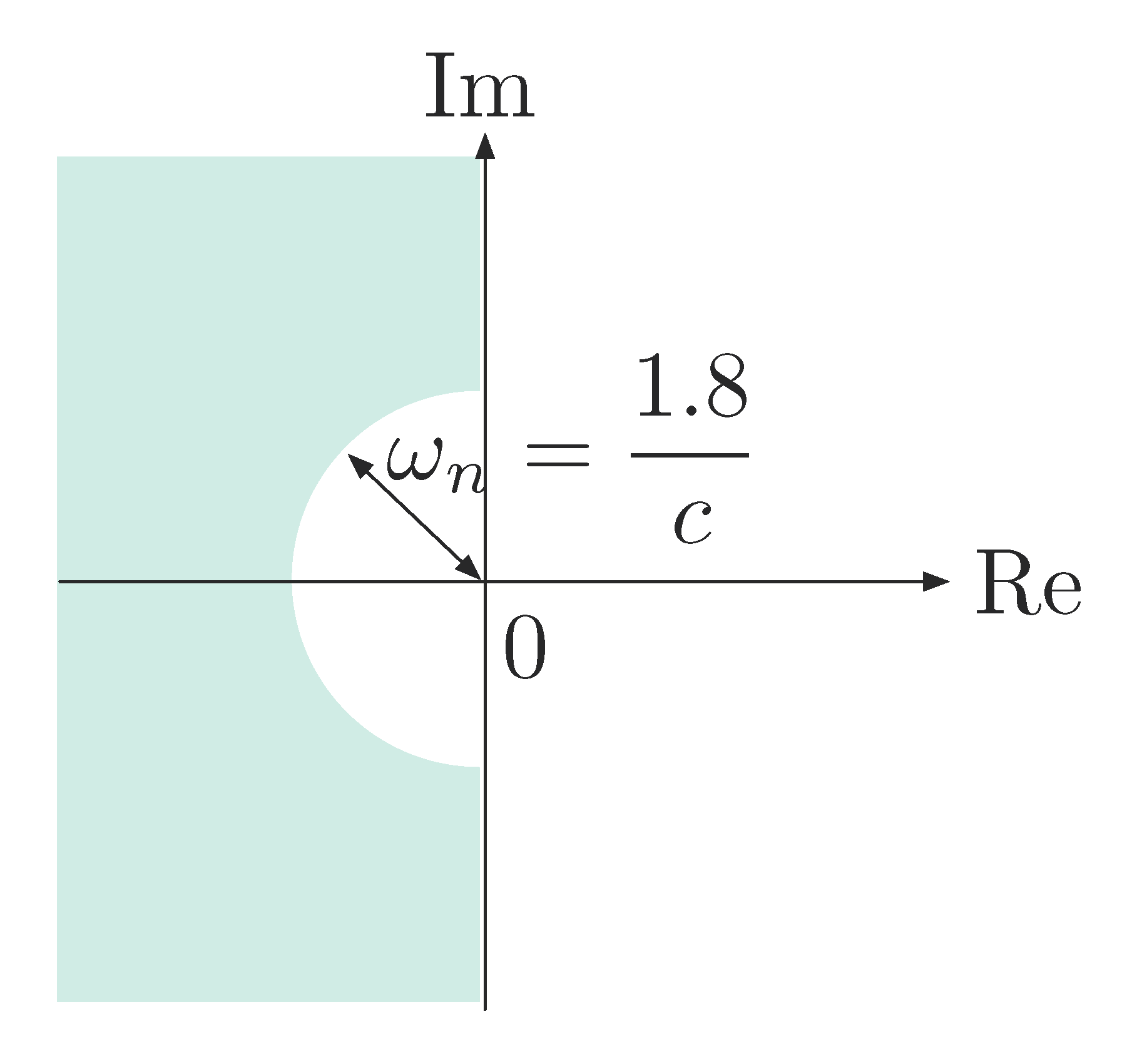
Figure 3: Possible pole locations in shaded region when \(t_r \le c\)
Constraints on Overshoot
Suppose we want \(M_p \le c\), by \[ M_p = \underbrace{\exp\left( - \dfrac{\pi\zeta}{\sqrt{1-\zeta^2}}\right)}_{\text{decreasing function}} \le c, \]
we need a large damping ratio. Furthermore, recall from last time,
\begin{align*} \frac{\zeta}{\sqrt{1-\zeta^2}} &= \frac{\omega_n\zeta}{\omega_n\sqrt{1-\zeta^2}} \\ &= \frac{\sigma}{\omega_d} \\ &= \cot \varphi, \end{align*}therefore \(\varphi\) shall be small. Geometrically, we want poles to lie in the shaded region as in Figure 4.
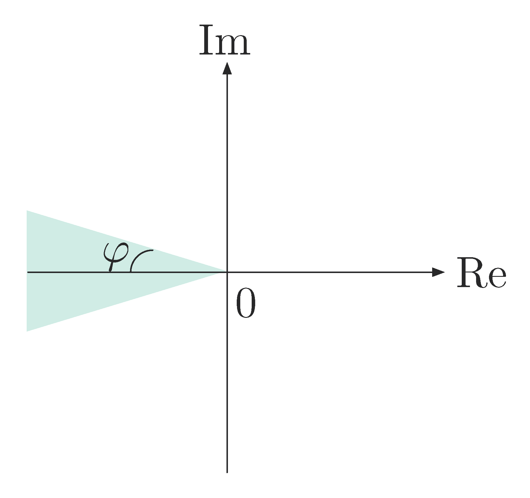
Figure 4: Possible pole locations in shaded region when \(M_p \le c\)
Intuition: A good damping ratio implies a good decay in roughly half a period.
Constraints on Settling Time
Suppose we want \(t_s \le c\), then
\begin{align*} t_s &\approx \dfrac{3}{\sigma} \le c \\ \implies &\sigma \ge \dfrac{3}{c}. \end{align*}Therefore the real part of poles \({\rm Re}(s) = - \sigma\) shall be large in terms of magnitude, i.e., far away from origin. Geometrically, we want poles to lie in the shaded region as in Figure 5.
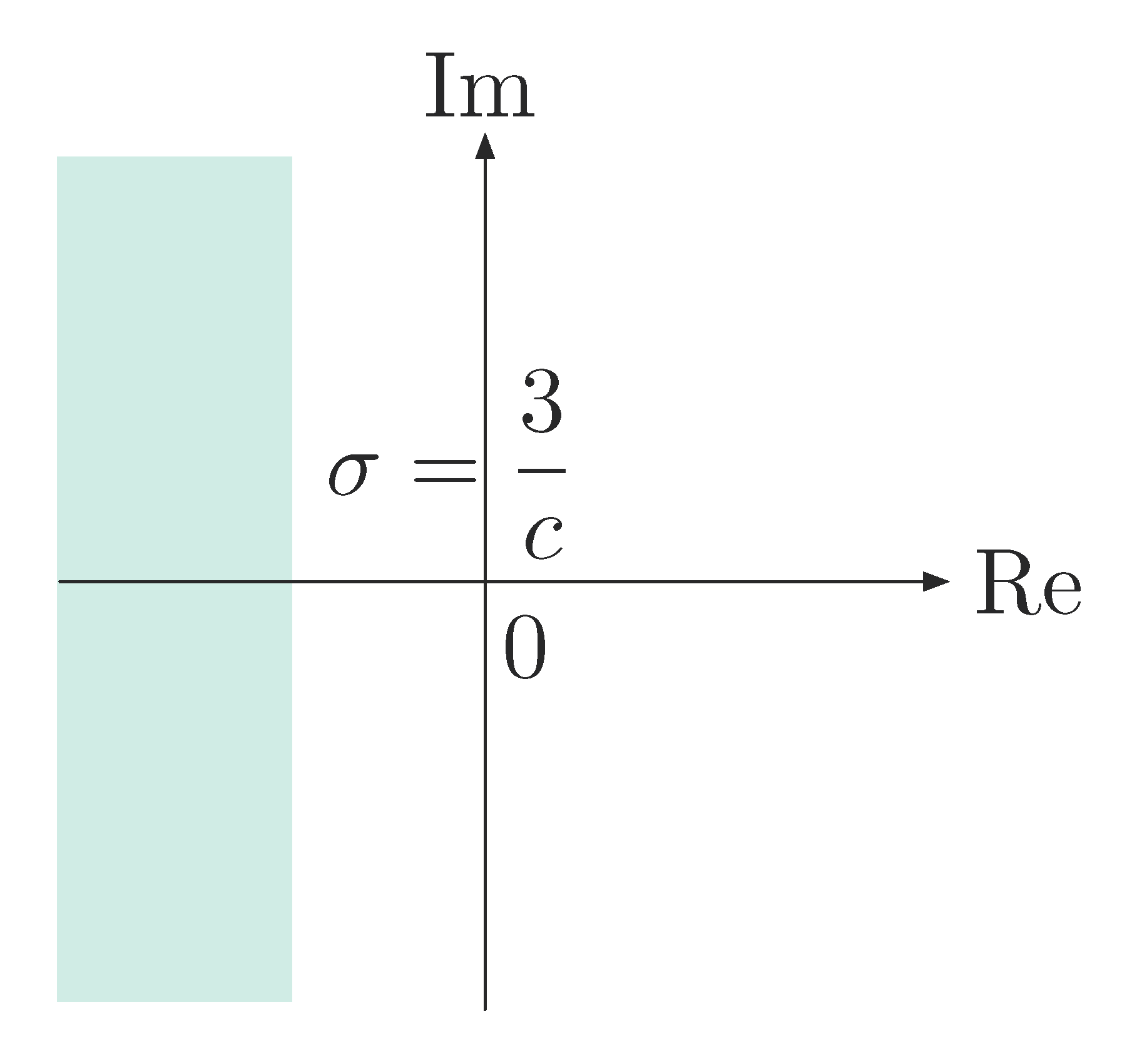
Figure 5: Possible pole locations in shaded region when \(t_s \le c\)
Intuition: Poles that are deep into the Left Half Plane (LHP) implies transients decay fast, i.e., overall \(t_s\) is smaller.
Combination of Constraints on Rise Time, Overshoot, Settling Time
If we have specifications for combinations of \(t_r, M_p, t_s\), we can easily relate them to allowed pole locations as we did for each of them, only overlaying them on a single sheet.
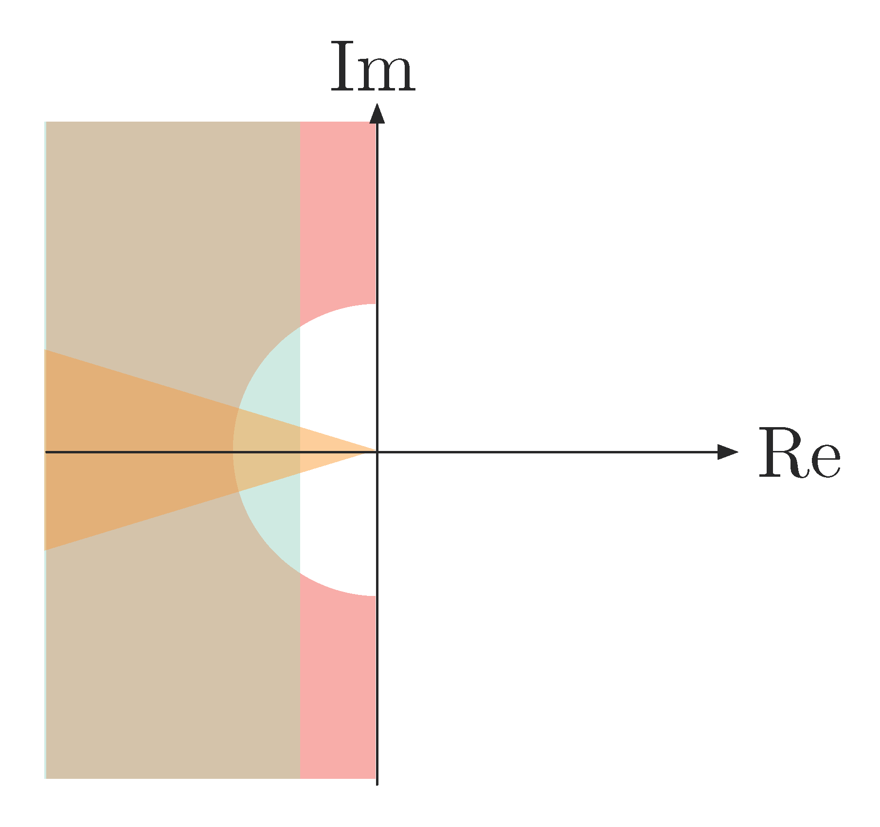
Figure 6: Possible pole locations in overlaid shaded region when \(t_r\), \(M_p\), \(t_s\) are constrained
The shape and size of the region for admissible pole locations will change depending on which specs are more severely constrained.
Note: Drawing sketches is very appealing to engineers since it is easy to visualize things, even though no such crisp visualization is easily available in time domain. But sketches are not very rigorous, let alone proofs. Also since we used approximations for prototype second order system, which has only two poles and no zeros, these geometric drawings are only valid in a very narrow range of scenarios.