CS357 NUMERICAL METHODS I
Summer 2014
Machine Problem 3
Posted: Monday July 28th , 2014
Due Date: 9:00 P.M., Wednesday, August 6h, 2014
This MP has three parts.
Handin is available here.
To run this MP you will need to use the following commands at the Linux prompt:
$ module load python3
$ easy_install-3.4 --user pillow
You will have to submit (using svn) the following files:
For Part 1:
compression.py
part1_answers.txt (answer to questions in Part 1)
For Part 2:
part2_answers.txt (answers to both questions in Section A of Part 2)
basic_powerpagerank.py
pagerank.py
powerpagerank.py
For Part 3:
adaptive.py
Part 1: (12 points) Image Compression Using SVD
Files used in Part 1 for this MP:
1. compression.py file – the Python file in which you will write your code for image compression
2. img.jpg – image you will be compressing
3. Now split the picture into three matrices Red, Green and Blue - How?
So split this matrix and name the variables Red, Green and Blue.
6. If display is True then show() the newImage.
8. Return rankRed and nrankRed
Report the new file size in the answers.txt file.
(grader: 4 points for compression.py running correctly without errors)
(grader: 8 points, 1 point for each of the eight blanks below.)
File size in bytes( use the unix ls –l command)
Rank 600: _____?____
Rank 800: _______?____
Part 2: (26 points) PageRank Algorithm
Section 1 : Understanding Page Rank (9 points)
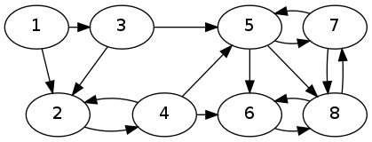
![]()
To compute the page rank I(P), we construct the matrix H, such that
![]()
Now, we can see that if I is the importance vector [I(Pi)],
![]()
Section 2 : Hyperlink matrix construction and using power method to compute page rank (12 points)
We shall examine the conditions and how it fails at the end of this section.
Implementation (basic_powerpagerank.py file)
Open the basic_powerpagerank.py file we provide you and enter your code to define the function:
def basic_powerpagerank(E, Ig, tol=1.0e-8, maxit=1000):
Ig is an initial guess of the importance vector I,
tol specifies the tolerance below which we assume convergence (default to 1.0e-8),
maxit specifies the maximum number of iterations after which we give up (default to 1000).
Step-by-step instructions to complete basic_powerpagerank is given below.
-
Step 0: Assign n to be the number of nodes, i.e., either number of rows or number of columns of E.
-
Step 1: Eliminate self-referential links, i.e., set the diagonal elements to be zero. (Can use np.diag())
-
Step 2: Calculate out-degree 'od' and in-degree 'id'. Out-degree is the number of links from a page P and in-degree is number of links to page P.
![]() , i.e., sum of the entries in column j of E.
, i.e., sum of the entries in column j of E.
![]() , i.e., sum of the entries in row i of E.
, i.e., sum of the entries in row i of E.
-
Step 3: Scale the matrix so each column sum is 1, if it was non-zero. Hint: You need to divide each column j by 1/od[j] if od[j] is not zero. This is the hyperlink matrix H.
-
Step 4: Use power method to find the eigenvector I. Starting with an initial value of I as Ig, compute HI. Terminate the loop if
◦ Maximum of the difference between two consecutive I is less than tol, or
◦ Number of iterations (iter) is greater than or equal to maxit.
-
Step 5: Scale the result I so that the sum is 1, only if sum is non-zero.
-
Step 6: Print “No convergence” if the convergence criterion was not met.
-
Step 7: Return the computed I and the number of iterations (iter).
To test your implementations, we have provided a utility function makeEdgeMat in the file util.py.
This function takes as input a filename containing graph information, and returns an edge matrix corresponding to the graph.
The graph can be specified by:
-
First line contains two integers, number of nodes n and number of edges e.
-
Following lines contain two integers n1, n2 (between 1 and n) such that there is an edge from Pn1 to Pn2.
-
# is for comments.
We have provided a few graph specifications too for your test cases.
To test, at the linux prompt, type:
$ module load python3
$ python3 basic_powerpagerank.py
Your code will be graded by passing the following tests.
Test 1: Normal execution
I = [ 0.06 0.0675 0.03 0.0675 0.0975 0.2025 0.18 0.295]
iterations = 96
(grader: 1 point)
( result for running
print("Test 1: Normal execution")
E = makeEdgeMat('graph1.dat')
Ig = np.ones(E.shape[0])/E.shape[0]
I, iter = basic_powerpagerank(E, Ig)
print('I =', I)
print('iterations =', iter, '\n') )
Test 2: Dangling node (all zero)
I = [ 0. 0.]
iterations = 3
(grader: 1 point)
( result for running
print("Test 2: Dangling node (all zero)")
E = makeEdgeMat('graph2.dat')
Ig = np.zeros(E.shape[0])
Ig[0] = 1
I, iter = basic_powerpagerank(E, Ig)
print('I =', I)
print('iterations =', iter, '\n') )
Test 3: Dangling node (unsatisfactory result)
I = [ 0. 0.]
iterations = 3
(grader: 1 point)
( result for running
print("Test 3: Dangling node (unsatisfactory result)")
E = makeEdgeMat('graph2.dat')
Ig = np.ones(E.shape[0])/E.shape[0]
I, iter = basic_powerpagerank(E, Ig)
print('I =', I)
print('iterations =', iter, '\n') )
Test 4: Loop (no convergence)
No convergence
I = [ 1. 0. 0. 0. 0.]
iterations = 1000
(grader: 1 point)
( result for running
print("Test 4: Loop (no convergence)")
E = makeEdgeMat('graph3.dat')
Ig = np.zeros(E.shape[0])
Ig[0] = 1
I, iter = basic_powerpagerank(E, Ig)
print('I =', I)
print('iterations =', iter, '\n') )
Test 5: Loop (valid convergence)
I = [ 0.2 0.2 0.2 0.2 0.2]
iterations = 1
(grader: 1 point)
( result for running
print("Test 5: Loop (valid convergence)")
E = makeEdgeMat('graph3.dat')
Ig = np.ones(E.shape[0])/E.shape[0]
I, iter = basic_powerpagerank(E, Ig)
print('I =', I)
print('iterations =', iter, '\n') )
Test 6: Sink (unsatisfactory result)
I = [ 0. 0. 0. 0. 0.12 0.24 0.24
iterations = 153
(grader: 1 point)
( result for running
print("Test 6: Sink (unsatisfactory result)")
E = makeEdgeMat('graph4.dat')
Ig = np.ones(E.shape[0])/E.shape[0]
I, iter = basic_powerpagerank(E, Ig)
print('I =', I)
print('iterations =', iter, '\n') )
Understanding your results
Graph G1 is represented by graph1.dat, which is used by Test 1.
As we can see, the algorithm terminates and provides a satisfactory page rank vector I.
Now, we have the following questions:
-
Does the sequence I k always converge?
-
Is the vector to which it converges independent of the initial vector Ig?
-
Do the importance ranking contain information that we want?
Let us examine the other test cases.
Test 2 and 3 use the graph G2, represented by graph2.dat.
Here, we just have two nodes and one edge. With initial value of Ig = [ 1 0 ] and Ig = [ 0.5 0.5 ], we got the resulting I to be [ 0 0 ], which says both the pages are not important at all, but this is not what we want their importance to be! This is because the node 2 has no outgoing edges, and hence acts like an importance sink, draining all the importance from 1.
Test 4 and 5 use the graph G3, represented by graph3.dat.
The graph here is a symmetric loop of 5 nodes. With an initial condition of [1 0 0 0 0 ], the algorithm does not converge, as you can see from test 4. To see what is happening to I, you can print I computed in each iteration (and reduce maxit so you don't see a lot of prints), and observe the pattern of I. This happens because we make the assumption in the power method that ![]() and
and ![]() . However, in this case,
. However, in this case, ![]() and thus, it does not converge for all starting vectors.
and thus, it does not converge for all starting vectors.
Test 5, uses an initial condition of [1/5 1/5 1/5 1/5 1/5] and converges to itself immediately.
Test 6 uses Graph G4, represented by graph4.dat.
The importance of the first 4 nodes is zero! This is because the second half behaves like an importance sink, similar to node 2 of G2, and drains the importance from the first half.
But, this is not a satisfactory result, as the first four nodes have edges and they should have some non-zero importance.
To answer our earlier questions,
-
Sequence I k does NOT always converge.
-
The vector to which it converges is NOT independent of the initial vector Ig.
-
The importance ranking does NOT always contain information we want.
Section C : Modifying the matrix to be stochastic and using matrix operations to obtain page rank (11 points)
The reason why our method fails, is because we want an irreducible and primitive stochastic matrix, but we don't necessarily have it always. To understand what that means, let us look at a probabilistic interpretation of H.
Imagine that we surf the web at random, i.e., when we are on a web page, we randomly pick any of its links to another page, and so on. So, if we are on page Pj with Ij links, if one of the pages it points to is Pi, the probability of opening Pi is 1/Ij.
Then, the fraction of time spent on page Pi can be interpreted to be its page rank I(Pi). Notice that, given this definition, we require the sum of page ranks to be 1.
Given this interpretation, we come to the first problem we saw before, the case of the dangling node. There are no edges from this node, then where do we go? Do we spend the rest of the time there?
To solve this problem, we will randomly choose any of the n pages. Thus, we replace all the entries in a column corresponding to a dangling node to be 1/n and call this new matrix S.
The matrix S has all its entries non negative, and sum of each column is 1. This is a stochastic matrix.
The second problem we faced was that ![]() and thus the eigenvector sequence I kdid not always converge. This is because the matrix H was not primitive. The matrix H to be primitive means , for some m, Hm has all positive entries. In other words, there is a way to get from the first page to the second page after following m links given two pages.
and thus the eigenvector sequence I kdid not always converge. This is because the matrix H was not primitive. The matrix H to be primitive means , for some m, Hm has all positive entries. In other words, there is a way to get from the first page to the second page after following m links given two pages.
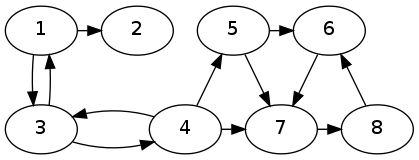
The third problem we faced was that matrix H was reducible, i.e., H can be written in block form as
![]()
To solve both these problems, i.e., to make S both primitive and irreducible, we need to modify the way our random surfer moves through the web. We consider a damping factor ![]() , such that the random surfer follows a link with the probability
, such that the random surfer follows a link with the probability ![]() , and chooses a random page with probability
, and chooses a random page with probability ![]() .
.
This theoretical random walk is known as a Marcov chain.
So, to obtain the Google matrix G,
![]()
Matrix G is the transition probability matrix of the Marcov chain and all its entries are non negative and sum of each column is 1. The matrix G is a primitive and irreducible stochastic matrix and has a stationary eigenvector I.
Then, ![]() can be written as
can be written as
![]()
where Id is n X n identity matrix, and e is an n vector of all ones. ![]() is a constant that varies with the sum of entries in I, and hence can be scaled to 1.
is a constant that varies with the sum of entries in I, and hence can be scaled to 1.
Thus, to compute the page ranks I, we need to solve the system of equations
![]()
Implementation (pagerank.py file)
Open the pagerank.py file provided and enter your code to define the function:
def pagerank(E, alpha):
where E is an edge matrix, such that![]() if there is a hyperlink from page Pj to Pi ,
if there is a hyperlink from page Pj to Pi ,
alpha is the damping factor to be considered.
Step-by-step instructions to complete pagerank is given below.
-
Step 0: Repeat steps 0 to 3 from section B to obtain the scaled hyperlink matrix H.
-
Step 1: Construct a matrix A such that all entries are zero except columns of dangling nodes, whose entries must be 1/n.
(Hint: Create an array a which has 1/n if od[i] is 0, 0 otherwise, and use np.vstack to make an n X n matrix)
-
Step 2: Form the stochastic matrix S to be H + A.
-
Step 3: Solve (Identity – alpha*S) I = e for I
(You can use np.eye() to create identity matrix, np.ones() to create a vector of all ones, np.linalg.solve() to solve the system of equations)
-
Step 4: Normalize vector I such that sum of entries is 1.
-
Step 5: Return I.
Test
To test, at the linux prompt, type:
$ module load python3
$ python3 pagerank.py
The first 4 test cases are provided for you. However, you must write your own edge matrix for test 5, for the following graph G5. (You can write a .dat file and use our util function, or write your edge matrix directly.)
Test 1: Stochastic
I = [ 0.06309315 0.09252519 0.04556459 0.09739641 0.11005375 0.18410088 0.15650523 0.2507608 ]
(grader: 1 point)
( result for running
print("Test 1: Stochastic")
E = makeEdgeMat('graph1.dat')
I = pagerank(E, 0.85)
print('I =', I, '\n') )
Test 2: Dangling node
I = [ 0.35087719 0.64912281]
(grader: 1 point)
( result for running
print("Test 2: Dangling node")
E = makeEdgeMat('graph2.dat')
I = pagerank(E, 0.85)
print('I =', I, '\n') )
Test 3: Loop (Not primitive)
I = [ 0.2 0.2 0.2 0.2 0.2]
(grader: 1 point)
( result for running
print("Test 3: Loop (Not primitive)")
E = makeEdgeMat('graph3.dat')
I = pagerank(E, 0.85)
print('I =', I, '\n') )
Test 4: Sink (reducible)
I = [ 0.01875 0.05715045 0.02671875 0.06732788 0.12848733 0.2056777 0.18660147 0.30928641]
(grader: 1 point)
( result for running
print("Test 4: Sink (reducible)")
E = makeEdgeMat('graph4.dat')
I = pagerank(E, 0.85)
print('I =', I, '\n') )
Test 5: Custom graph
I = [ 0.04768256 0.04365325 0.05716331 0.04768256 0.03689822 0.25121828 0.2661155 0.24958633]
(grader: 1 point)
( result for running
print("Test 5: Custom graph")
# write your code here
I = pagerank(E, 0.85)
print('I =', I, '\n') )
Section D : Using power method to obtain page rank for modified matrix (12 points)
In this section, we combine your work from section B and C to obtain the page rank from the modified google matrix G using power method, and check the effect of ![]() on the convergence.
on the convergence.
When ![]() is 1, G = S, which is just a stochastic matrix which could be reducible and not primitive. When
is 1, G = S, which is just a stochastic matrix which could be reducible and not primitive. When ![]() is 0, it makes the matrix all 1/n, thus the importance of each page is equal to 1/n and we lose the structural information of the graph. Thus, we want
is 0, it makes the matrix all 1/n, thus the importance of each page is equal to 1/n and we lose the structural information of the graph. Thus, we want ![]() to be as high as possible to retain structural information but not 1 as the algorithm will not always converge. Also, it can be proven that the second eigenvalue
to be as high as possible to retain structural information but not 1 as the algorithm will not always converge. Also, it can be proven that the second eigenvalue ![]() , and with high
, and with high ![]() , the algorithm takes longer to converge (from class).
, the algorithm takes longer to converge (from class).
We will test the effect of varying ![]() on the number of iterations it takes for convergence.
on the number of iterations it takes for convergence.
Implementation (powerpagerank.py file)
Open the powerpagerank.py file provided and enter your code to define the function:
def powerpagerank(E, alpha, Ig, tol=1.0e-8, maxit=1000):
where E is an edge matrix, such that![]() if there is a hyperlink from page Pj to Pi ,
if there is a hyperlink from page Pj to Pi ,
alpha is the damping factor to be considered,
Ig is an initial guess of the importance vector I,
tol specifies the tolerance below which we assume convergence (default to 1.0e-8),
maxit specifies the maximum number of iterations after which we give up (default to 1000).
Step-by-step instructions to complete pagerank is given below.
-
Step 0: Repeat steps 0 to 2 from section C to obtain the stochastic matrix S.
-
Step 1: Compute G = alpha*S + (1 – alpha)*O/n, where O is an n X n matrix of all ones.
(Can use np.ones() to create nXn matrix of ones)
-
Step 2: Repeat steps 4 to 7 from section B using G instead of H to compute and return I and iter.
Test
To test, at the linux prompt, type:
$ module load python3
$ python3 powerpagerank.py
Update test 5 by copying the code for E from pagerank.py (section C).
Test 1: Stochastic
I = [ 0.06309315 0.09252519 0.04556459 0.09739641 0.11005375 0.18410088 0.15650523 0.2507608]
iterations = 45
(grader: 1 point)
( result for running
print("Test 1: Stochastic")
E = makeEdgeMat('graph1.dat')
Ig = np.ones(E.shape[0])/E.shape[0]
I, iter = powerpagerank(E, 0.85, Ig)
print('I =', I)
print('iterations =', iter, '\n') )
Test 2: Dangling node
I = [ 0.35087719 0.64912281]
iterations = 23
(grader: 1 point)
( result for running
print("Test 2: Dangling node")
E = makeEdgeMat('graph2.dat')
Ig = np.zeros(E.shape[0])
Ig[0] = 1
I, iter = powerpagerank(E, 0.85, Ig)
print('I =', I)
print('iterations =', iter, '\n') )
Test 3: Loop (Not primitive)
I = [ 0.20000001 0.2 0.2 0.2 0.2]
iterations = 115
(grader: 1 point)
( result for running
print("Test 3: Loop (Not primitive)")
E = makeEdgeMat('graph3.dat')
Ig = np.zeros(E.shape[0])
Ig[0] = 1
I, iter = powerpagerank(E, 0.85, Ig)
print('I =', I)
print('iterations =', iter, '\n') )
Test 4: Sink (reducible)
I = [ 0.01875 0.05715045 0.02671875 0.06732788 0.12848733 0.2056777 0.18660147 0.30928642]
iterations = 57
(grader: 1 point)
( result for running
print("Test 4: Sink (reducible)")
E = makeEdgeMat('graph4.dat')
Ig = np.ones(E.shape[0])/E.shape[0]
I, iter = powerpagerank(E, 0.85, Ig)
print('I =', I)
print('iterations =', iter, '\n') )
Test 5: Custom graph
I = [ 0.04768256 0.04365325 0.05716331 0.04768256 0.03689822 0.25121827 0.2661155 0.24958633]
iterations = 98
(grader: 1 point)
( result for running
print("Test 5: Custom graph")
# write your code here
Ig = np.ones(E.shape[0])/E.shape[0]
I, iter = powerpagerank(E, 0.85, Ig)
print('I =', I)
print('iterations =', iter, '\n') )
alpha iterations
0.05 6
0.10 7
0.15 9
0.20 10
0.25 12
0.30 14
0.35 16
0.40 18
0.45 20
0.50 23
0.55 27
0.60 31
0.65 37
0.70 45
0.75 55
0.80 71
0.85 98
0.90 150
0.95 308
(grader: 1 points)
( result for running
print('Test 6: Effect of alpha on number of iterations')
print('alpha\titerations')
for alpha in np.arange(0.05, 1.00, 0.05):
I, iter = powerpagerank(E, alpha, Ig)
print('{0:3.2f}\t{1:5d}'.format(alpha, iter)) )
Part 3 (12 points): Adaptive Integration.
Instructions:
In this portion of the MP, we will be writing Python code to compute the definite integral

using the recursive method called adaptive integration. First we use the trapezoidal rule to perform the integration over an interval [a,b], for a given function y=f(x). For example see the figure below that shows a trapezoid with A_approx = (1/2)*(f(a)+f(b))*(b-a) = (f(0)+f(1))/2 where a = 0 , b=1 and f(x) = x2+2.
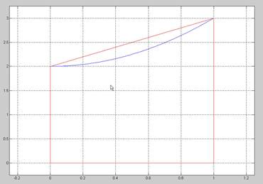
If the difference between the true area (A) and the area obtained by using the trapezoidal method (A_approx) is small we are done. But if we don't know A then how can we know that A_approx is good? One way to test our approximation is to subdivide the x axis into two intervals [a (a+b)/2] and [(a+b)/2, b] (or [0 1/2] and [1/2 1] in our problem) and form two trapezoids (as shown in the figure below).
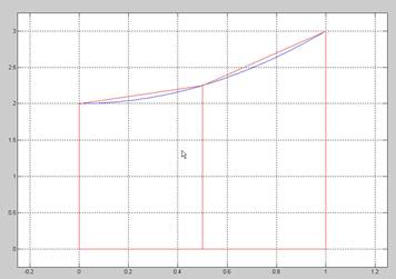
Our method is to compare the sum of the areas of the left trapezoid and the right trapezoid AL_approx + AR_approx with the area of the single trapezoid A_approx and if the difference is small then we are done. If the difference isn't small then we will use recursion applied to AL and AR respectively.
The idea explained above has been implemented in the Python function “adaptive.py”. You will have to complete this function and run the tests.
Open the Python function adaptive.py .
This file contains the following lines of code:
def adaptive(f, a, b, N, xlim, tol):

# integrafes f from a to b using N point trapezoid rule

# xlim denotes the x limits for the plot
    x = np.linspace(a, b, N)

    y = f(x)

    pt.fill_between(x, 0, y, facecolor='g')

    pt.xlim(xlim)

    pt.draw()

    pt.show(block=False)

    time.sleep(0.1)

    A = np.trapz(y, x)
# Find Al - Area of left half using N point trapezoid rule
# Find Ar - Area of right half using N point trapezoid rule
    if abs((Al + Ar) - A) < tol:

        pt.fill_between(x, 0, y, facecolor='r')

        pt.draw()

        return # The area

    else:

        return # Sum of recursively computed area of left half and right
Complete the code as per the comments in the code and then test your code.
To test your code, at the Linux prompt type the following.
$ module load python3
$ python3 adaptive.py
Tests
(grader: 3 points for each of the following four tests for a total of 12 poitns for Part 3)
integral x^2 from 0 to 1
Area = 0.33349609375
integral x^3 from 0 to 1
Area = 0.250000489163
integral sin(x) from 0 to pi/2
Area = 0.999999999787
integral xx2 from 0 to 2
Area = 2.83333534272