Gan
IE 534 - Understanding CNNs and Generative Adversarial Networks
The assignment consists of training a Generative Adversarial Network on the CIFAR10 dataset as well as a few visualization tasks for better understanding how a CNN works.
- Train a baseline model for CIFAR10 classification (~2 hours training time)
- Train a discriminator/generator pair on CIFAR10 dataset utilizing techniques from ACGAN and Wasserstein GANs (~40-45 hours training time)
- Use techniques to create synthetic images maximizing class output scores or particular features as a visualization technique to understand how a CNN is working (<1 minute)
This homework is slightly different than previous homeworks as you will be provided with a lot of code and sets of hyperparameters. You should only need to train the models once after you piece together the code and understand how it works. The second part of the homework (feature visualization) utilizes the models trained from part 1. The output will need to be run many times with various parameters but the code is extremely fast.
The assignment is written more like a tutorial. The Background section is essentially a written version of the lecture and includes links to reference materials. It is very important to read these. Part 1 will take you through the steps to train the necessary models. Part 2 will take you through the steps of getting output images which are ultimately what will be turned in for a grade. Parts 1 and 2 will make frequent references to the background section.
Make sure to load the more recent pytorch version. Some of the code may not work if you learn the default version on BlueWaters.
module load bwpy/2.0.0-pre2
Additionally, when using the Adam optimizer. There is sometimes an overflow issue when training for a large number of epochs. You may need to include this during training to prevent it from happening.
for group in optimizer.param_groups:
    for p in group['params']:
        state = optimizer.state[p]
            if('step' in state and state['step']>=1024):
                state['step'] = 1000
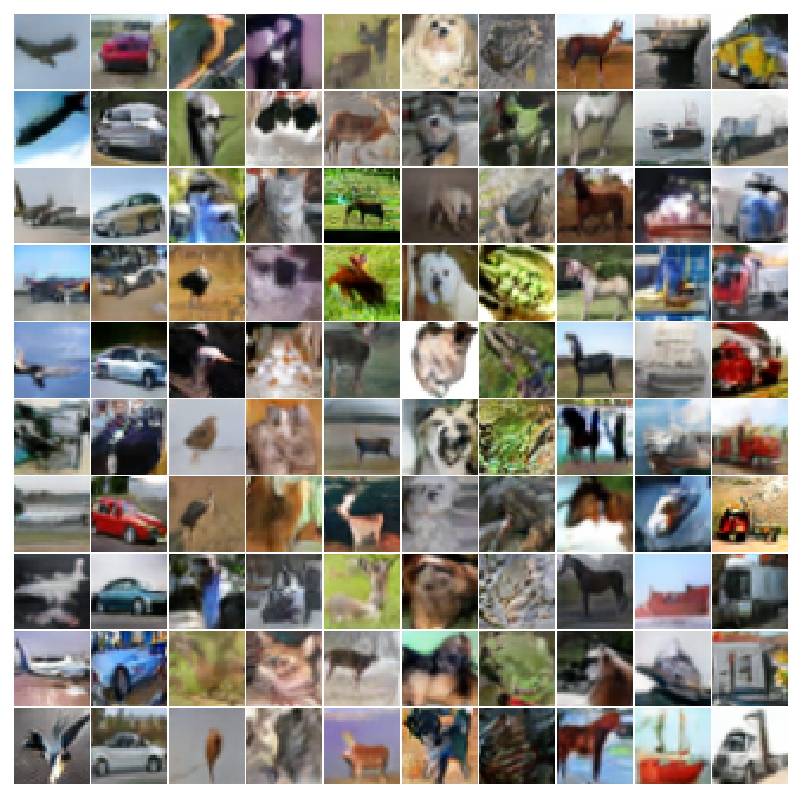
 Fake images generated from random noise to look like the CIFAR10 dataset. Each column is a class specific generation. Airplane, Car, Bird, Cat, Deer, Dog, Frog, Horse, Ship, Truck
Background
Discriminative vs Generative Models
Read the short wikipedia page if you’re unfamiliar with these terms
A generative method attempts to model the full joint distribution P(X,Y). For classification problems, we want the posterior probability P(Y|X) which can be gotten from the modeled P(X,Y) with Bayes’ Rule. In a similar fashion, we can also get the likelihood P(X|Y).
As an example, let X be a random variable for shoe size with Y being a label from {male,female}. Shoe size is a multi-modal distribution that can be modeled as two separate Gaussian distributions: one for male and one for female.
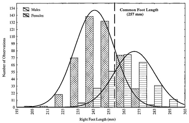
If provided with a particular shoe size as a classification task, the plot above shows easily how one could estimate P(Y|X). If an application requires it, a generative model could also generate fake data that looks real by sampling from each individual likelihood distribution P(X|Y). As long as the underlying distribution chosen for the modeling the data is correct (two independent Gaussians in this case), the sampled data is indistinguishable from the true data.
Neural networks for classification are trained in a discriminative fashion via SGD to model a pseudo-posterior probability P(Y|X) directly. This is not technically a true distribution although it is very useful in practice since the underlying data distributions are usually of high complexity with many modes. There isn’t necessarily a simple distribution like a Gaussian to easily describe it. The network is simply being provided with a large number of data pairs (X,Y) and attempts to learn some mathematical function capable of discriminating between the labels.
What if the application required the generation of realistic samples? By skipping ahead and only modeling P(Y|X), typical classification networks are not directly suited for generating samples matching the joint distribution P(X,Y) or individual likelihoods P(X|Y). Generative Adversarial Netowrks (GANs) are an attempt to capture benefits of generative models while still utilizing the successful techniques used for training discriminative neural networks.
Generative models are useful for things like:
- Representing and manipulating high dimensional probability distributions
- Reinforcement learning applications where the model generates “realistic” experiences to learn from when acquiring data may be costly.
- Unsupervised/Semi-Supervised learning (acquiring unlabeled data is typically easier)
- Capable of handling multi-modal models
 Lotter, W., Kreiman, G., and Cox, D. (2015). Unsupervised learning
of visual structure using predictive generative networks. arXiv preprint
arXiv:1511.06380 .
Lotter, W., Kreiman, G., and Cox, D. (2015). Unsupervised learning
of visual structure using predictive generative networks. arXiv preprint
arXiv:1511.06380 .
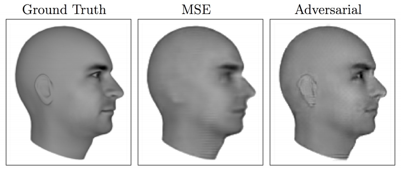
The above image is an example of a model attempting to predict the next frame of a 3d rendered moving face. The MSE predicts a “blurry” version of the many possible face positions that could be the next frame. With an additional GAN loss (a discriminator network deciding if it’s a ground truth image or from the generator), the generator is forced to choose one of the many possible positions while maintaining the sharp/detailed look of the ground truth.
Understanding CNNs (What does a CNN actually learn?)
In order generate realistic images with a GAN, it would help to understand a bit more about how CNNs work. For a problem like classification, what does it learn? Does it learn small or large objects? Does it learn larger objects are a collection of smaller parts? Does it have the concept of a “whole”? Consider how one might describe an objects’ looks to another person. Would a CNN have a similar description?
There are lot of questions to ask yourself while designing a network (input resolution, how many layers, how many hidden units, when to use pooling/stride, etc.) and there is no definitive answer. It’s true that a network will attempt to learn a mapping function from input to output during SGD without user input but the network needs to be capable of learning the appropriate mathematical functions before learning even begins. If the labels can only be discriminated by high resolution, complex patterns taking up large amounts of the input image, using large kernels with significant pooling could inhibit its ability to learn as opposed to a series of small kernel convolutions.
A network trained with SGD is only set up to discriminate between objects. It will not learn what it doesn’t need. It can also easily learn patterns in specific images that don’t generalize well across samples (overfitting). If your only output classes are a tiger and a soccerball, the network may only need to learn a single kernel capable of detecting orange. It outputs tiger if it sees orange and soccerball otherwise. If you add in a class for basketball, maybe it needs to also learn a straight stripe pattern and a zig zag pattern. Add another class for zebra and it now needs to differentiate between the colors of the stripes. The intuition follows that the more classes the model needs to discriminate between, the more its necessary for it to learn the concept of a “whole”. Additionally, with larger datasets, the more the network must use the features it has more efficiently such that there is overlap between classes which can help prevent overfitting.
The features of each layer as the input passes deeper into the network start off as simple patterns (edges, colors, etc.) and become more complex. Due to the nature of convolutions, the receptive field becomes larger allowing the features to become larger in the context of the original input image.
Receptive Field
The receptive field is the region of the input image that went into the calculation of a particular feature. The output of a convolution layer applied to an image is technically another image. Each pixel in this new image can only see a portion of the previous image. It is easy to see how after applying a kernel of size 3 would result in a new image where each pixel has a receptive field of 3x3. A subsequent convolution would result in another image with a receptive field of 5x5 compared to the original input.
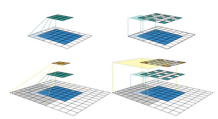
The image above shows how the receptive field grows when an input image of size 5x5 gets passed through a convolution layer with a kernel of 3, padding of 1, and a stride of 2. The left column shows the feature maps after each convolution. The right column adds blank spots in to show the stride with the color shaded regions signifying the size of the receptive field.
Convolutions, strided convolutions, and pooling layers affect the receptive field in different ways. Near the output of the network, the receptive field should be relative to the “size” of the objects of interest within the image.
This link here provides a more in depth explanation and is where the above picture is pulled from. It also shows explicit equations for how to calculate the receptive field. This link shows how the receptive field grows as the network gets deeper. The particular network shown in the link is the one you will create for this homework. Note the receptive field is 45x45 at the output which is larger than the CIFAR10 images (32x32). This means the features should be capable of capturing full objects.
Feature Visualization
It is possible to visualize the features and see how they become more interesting and complex as the network deepens. One method is to input a noisy initialized image and calculate the gradient of a particular feature within the network with respect to the input. This gradient indicates how changes in the input image affect the magnitude of the feature. This process can be repeated with the image being adjusted slightly each time with the gradient. The final image is then a synthesized image causing a very high activation of that particular feature.
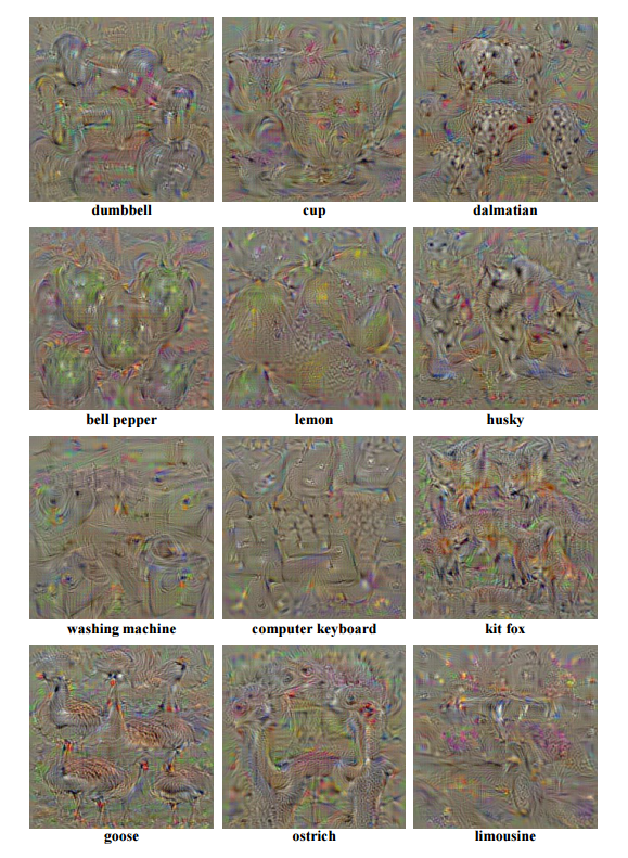
The above images are generated by backpropagating the error from the final classification layer for particular classes. These images do not look real but there are certain distinctive features. There are sometimes multiple outlines of the various objects, there are clear patterns associated with the objects (dots for the dalmation, squares for the computer keyboard, body outlines for the animals), and the size of the objects vary in terms of receptive field. There are lots of random points/colors/contours that cause high activation but not what we as humans would necessarily think are important.
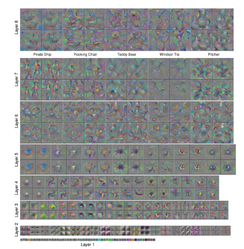
The following link goes much more in depth to this process and has references to a paper/visualization tool. You will do this for the second part of this assignment.
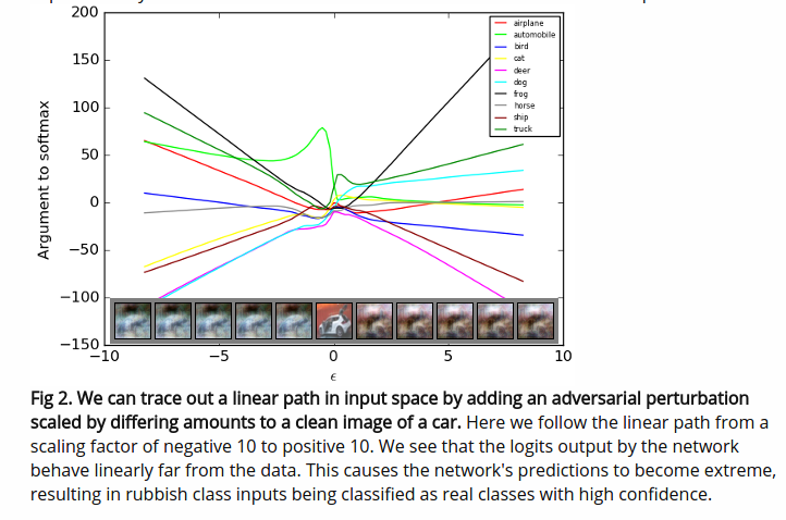
Tricking Networks
Similar to the feature visualization technique, real images correctly classified by a network can be imperceptibly altered to produce a highly confident incorrect output. Backpropagate the error for an alternative label to real image, use the sign of the gradient (-1 or 1), multiply this by 0.0078, and add it to the original image. A value of 0.0078 is 1⁄255 which is how colors are discretized for storing a digital image. Changing the value of the input image by less than this is imperceptible to humans but convolution networks can be highly sensitive to these changes.
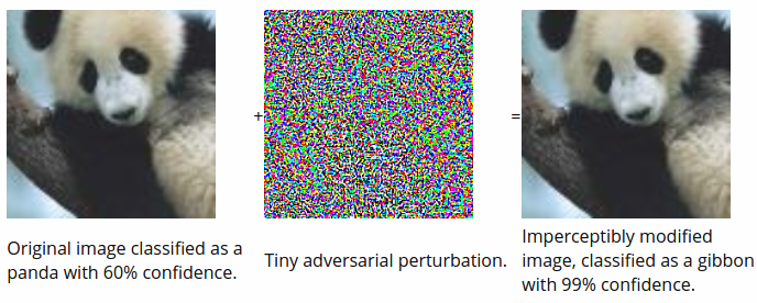
The above images are from this blog post written by the author of the original GAN paper, Ian Goodfellow.
Generative Adversarial Networks (GANs)
Slides 33-56 of the lecture notes already cover GANs as well as Wasserstein GANs. The explicit equations can be found there. It is heavily recommended to read the original GAN tutorial written by Ian Goodfellow as part of the assignment.
GANs consist of two separate networks typically referred to as the generator network and the discriminator network (refered to as the critic network in the Wasserstein GAN paper). The generator is capable of creating fake images from random noise. The discriminator is optimized to differentiate between real images and the images from the generator. The generator is provided with the gradient from the discriminator and is optimized to create fake images the discriminator considers real.
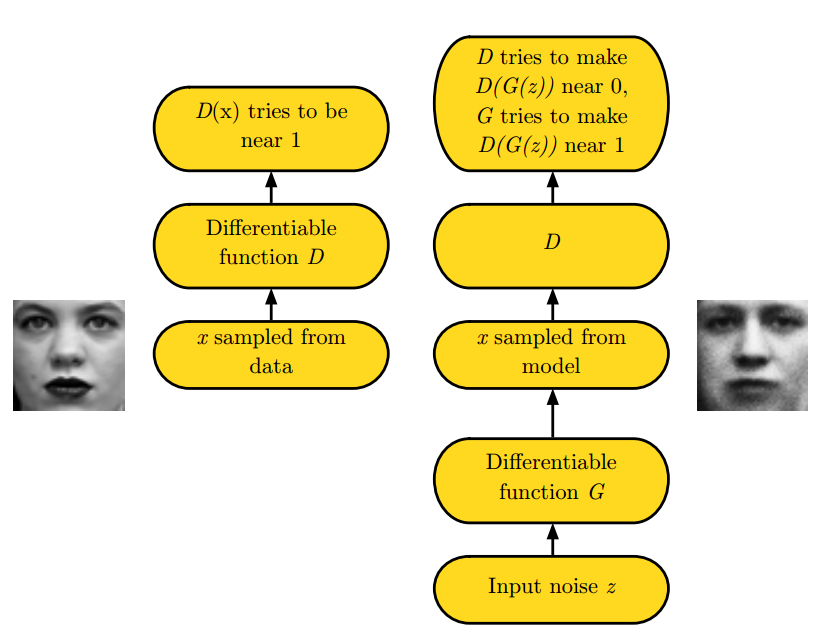
The discriminator is simply any convolutional neural network such as the ones used in previous assignments. The generator samples a vector from a random distribution and manipulates it with transposed convolutions until it is in the shape of an input image.
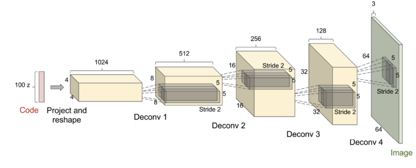
The above image is from the paper Unsupervised Representation Learning with Deep Convolutional Generative Advserial Networks and is typically referred to as DCGAN for short. Although they’re labeled as deconvolutions, the correct name is a transposed convolution as a deconvolution technically means the inverse of a convolution. The term deconvolution is sometimes seen in the literature.
Transposed Convolution
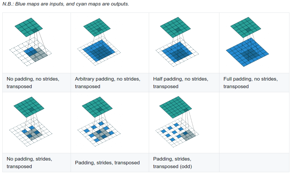
When a transposed convolution is used with a stride larger than 1, the output image is increases in size (bottom row of the above image). Animations for the above images can be found here as well as a technical document about convolutions. Transposed convolutions are discussed in chapter 4.
Auxiliary Classifer GAN (ACGAN)
The original GAN formulation was used for unsupervised learning and did not take into account any labels for the data. The final output from the discriminator was of dimension 1 representing the probability of the input being real. Conditional Image Synthesis with Auxiliary Classifier GANs introduced a technique for generating class specific examples by including an auxiliary classifier in the discriminator.
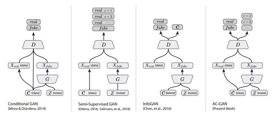
There are two primary distinctions. The first is the generator is provided with some information about the class label. When randomly generating a vector of length d for the generator, the first n dimensions (where n is the number of classes) are made to be 0.0 except for a 1.0 in the location of a randomly sampled class. Additionally, the discriminator has two separate output layers. The first is used as the critic for determining if the input is real or fake. The second is called the auxiliary classifier and has an output dimension equal to n which determines which class the input belongs to. During optimization, both the generator and the discriminator have an additional loss term which is simply the cross entropy error of the auxiliary classifier.
After training, this provides the additional benefit of being able to specify which class the generator should generate by placing a 1.0 in one of the first n dimensions of the randomly sampled vector.
Wasserstein GANs
The original GAN formulation had issues with training stability and the Wasserstein GAN helped address this problem. The Wasserstein GAN optimizes a different loss function. From an implementation standpoint, the only two changes are to remove the sigmoid operation from the final layer to directly be used for optimization and to introduce weight clipping to satisfy the Lipschitz constraint.
Improved Training for Wasserstein GANs found that weight clipping to enforce the Lipschitz constraint still led to undesired behavior. They penalize the norm of the gradient of the critic (discriminator) with the respect to its input to enforce the constraint instead with significantly improved results.
Batch normalization is typically used in both the generator and the discriminator networks. However, batch normalization causes the entire batch of outputs to be dependent on the entire batch of inputs which makes the gradient penalty invalid. Layer normalization is used as a replacement.
Layer Normalization
Layer Normalization attempted to address certain issues related to applying batch normalization to recurrent neural networks and to remove the batch dependencies between the input and output.
Let X be a data matrix of size b by d where b is the batch size and d is the number of features. Each row of this matrix is a separate sample of features. Each column is a single feature over the entire batch. Batch normalization normalizes with respect to the columns while layer normalization normalizes with respect to the row. Therefore, with layer normalization, the features of a single sample are normalized based on all of the other features in that sample without any information about other samples in the batch. This means the output from layer normalization is the same during the training and test phase.
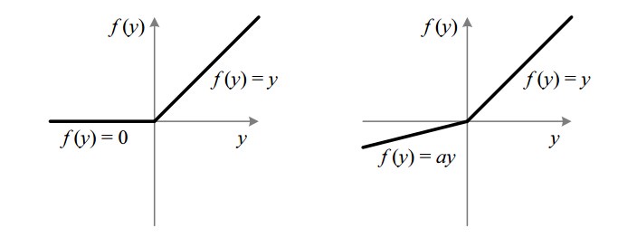
Leaky ReLU
It is typically easier to train GANs when a leaky ReLU is used in place of all ReLU activations in the discriminator. A leaky ReLU still allows gradient flow (albeit scaled down) even if the output is negative.
Part 1 - Training a GAN on CIFAR10
Note - I was mistaken about how long the generator trained with the discriminator should take (I originally said 30 hours). I seem to be getting variable performance on BlueWaters. The original networks I have defined below look like they will take around 90 hours. You have two options:
Use 128 features instead of 196 in both the generator and the discriminator. This should drop training time to around 43 hours for 400 epochs. The results look slightly worse but there isn’t much of a difference. The rest of the assignment should be the exact same.
Use 196 features but only train for 200 epochs. This should take around 42 hours.
As you will see after training, the results look “decent” after far less than than the required number of epochs. However, it does seem to slowly improve the longer you train.
Defining the Generator and Discriminator
| name | type | input_channels | output_channels | ksize | padding | stride | input | output |
|---|---|---|---|---|---|---|---|---|
| conv1 | conv2d | 3 | 196 | 3 | 1 | 1 | 32x32 | 32x32 |
| conv2 | conv2d | 196 | 196 | 3 | 1 | 2 | 32x32 | 16x16 |
| conv3 | conv2d | 196 | 196 | 3 | 1 | 1 | 16x16 | 16x16 |
| conv4 | conv2d | 196 | 196 | 3 | 1 | 2 | 16x16 | 8x8 |
| conv5 | conv2d | 196 | 196 | 3 | 1 | 1 | 8x8 | 8x8 |
| conv6 | conv2d | 196 | 196 | 3 | 1 | 1 | 8x8 | 8x8 |
| conv7 | conv2d | 196 | 196 | 3 | 1 | 1 | 8x8 | 8x8 |
| conv8 | conv2d | 196 | 196 | 3 | 1 | 2 | 8x8 | 4x4 |
| pool | max2d | 4 | 0 | 4 | 4x4 | 1x1 | ||
| fc1 | linear | 196 | 1 | |||||
| fc10 | linear | 196 | 10 |
Use the table above to create a PyTorch model for the discriminator. This is similar to classification networks created in previous homeworks. Use Layer Normalization after every convolution operation followed by a Leaky ReLU. There are built in PyTorch implementations for both of these. Unlike batch normalization, layer normalization needs the width and height of its input as well as the number of features. Notice there are two fully connected layers. Both have the same input (the output from the pool operation). fc1 is considered the output of the “critic” which is a score determining of the input is real or a fake image coming from the generator. fc10 is considered the auxiliary classifier which corresponds to the class label. Return both of these outputs in the forward call.
| name | type | input_channels | output_channels | ksize | padding | stride | input | output |
|---|---|---|---|---|---|---|---|---|
| fc1 | linear | 100 (noise) | 196*4*4 | |||||
| conv1 | convtranspose2d | 196 | 196 | 4 | 1 | 2 | 4x4 | 8x8 |
| conv2 | conv2d | 196 | 196 | 3 | 1 | 1 | 8x8 | 8x8 |
| conv3 | conv2d | 196 | 196 | 3 | 1 | 1 | 8x8 | 8x8 |
| conv4 | conv2d | 196 | 196 | 3 | 1 | 1 | 8x8 | 8x8 |
| conv5 | convtranspose2d | 196 | 196 | 4 | 1 | 2 | 8x8 | 16x16 |
| conv6 | conv2d | 196 | 196 | 3 | 1 | 1 | 16x16 | 16x16 |
| conv7 | convtranspose2d | 196 | 196 | 4 | 1 | 2 | 16x16 | 32x32 |
| conv8 | conv2d | 196 | 3 | 3 | 1 | 1 | 32x32 | 32x32 |
Use the table above to create a PyTorch model for the generator. Unlike the discriminator, ReLU activation functions and batch normalization can be used. Use both of these after every layer except conv8. This last layer is outputting a 32x32 image with 3 channels representing the RGB channels. This is fake image generated from the 100 dimensional input noise. During training, the real images will be scaled between -1 and 1. Therefore, send the output of conv8 through a hyperbolic tangent function (tanh). Also, take notice the transposed convolution layers. There is a built in PyTorch module for this.
Train the Discriminator without the Generator
This part is no different than homework 3 except you will need to train the discriminator defined above.
transform_train = transforms.Compose([
    transforms.RandomResizedCrop(32, scale=(0.7, 1.0), ratio=(1.0,1.0)),
    transforms.ColorJitter(
            brightness=0.1*torch.randn(1),
            contrast=0.1*torch.randn(1),
            saturation=0.1*torch.randn(1),
            hue=0.1*torch.randn(1)),
    transforms.RandomHorizontalFlip(),
    transforms.ToTensor(),
    transforms.Normalize((0.5, 0.5, 0.5), (0.5, 0.5, 0.5)),
])

transform_test = transforms.Compose([
    transforms.CenterCrop(32),
    transforms.ToTensor(),
    transforms.Normalize((0.5, 0.5, 0.5), (0.5, 0.5, 0.5)),
])

trainset = torchvision.datasets.CIFAR10(root='./', train=True, download=True, transform=transform_train)
trainloader = torch.utils.data.DataLoader(trainset, batch_size=batch_size, shuffle=True, num_workers=8)

testset = torchvision.datasets.CIFAR10(root='./', train=False, download=False, transform=transform_test)
testloader = torch.utils.data.DataLoader(testset, batch_size=batch_size, shuffle=False, num_workers=8)
Use the above code for the train and test loader. Notice the normalize function has mean and std values of 0.5. The original dataset is scaled between 0 and 1. These values will normalize all of the inputs to between -1 and 1 which matches the hyperbolic tangent function from the generator.
model =  discriminator()
model.cuda()
criterion = nn.CrossEntropyLoss()
optimizer = torch.optim.Adam(model.parameters(), lr=0.0001)
Create a train and test loop as done in homework 3. I trained the model for 100 epochs with a batch size of 128 and dropped the learning rate at epochs 50 and 75. Make sure the model outputs the train/test accuracy so you can report it later. It should achieve between 87%-89% on the test set.
if(epoch==50):
    for param_group in optimizer.param_groups:
        param_group['lr'] = learning_rate/10.0
if(epoch==75):
    for param_group in optimizer.param_groups:
        param_group['lr'] = learning_rate/100.0
Depending on how you set up the return function in the discriminator, only use the fc10 output. The fc1 output can be ignored for now.
for batch_idx, (X_train_batch, Y_train_batch) in enumerate(trainloader):

    if(Y_train_batch.shape[0] < batch_size):
        continue

    X_train_batch = Variable(X_train_batch).cuda()
    Y_train_batch = Variable(Y_train_batch).cuda()
    _, output = model(X_train_batch)

    loss = criterion(output, Y_train_batch)
    optimizer.zero_grad()

    loss.backward()
    optimizer.step()
Lastly, make sure to save the model after training. This will be used later in Part 2.
torch.save(model,'cifar10.model')
Train the Discriminator with the Generator
Training a GAN takes significantly longer than training just the discriminator. For each iteration, you will need to update the generator network and the discriminator network separately. The generator network requires a forward/backward pass through both the generator and the discriminator. The discriminator network requires a forward pass through the generator and two forward/backward passes for the discriminator (one for real images and one for fake images). On top of this, the model can be trained for a large number of iterations. I trained for 500 epochs.
def calc_gradient_penalty(netD, real_data, fake_data):
    DIM = 32
    LAMBDA = 10
    alpha = torch.rand(batch_size, 1)
    alpha = alpha.expand(batch_size, int(real_data.nelement()/batch_size)).contiguous()
    alpha = alpha.view(batch_size, 3, DIM, DIM)
    alpha = alpha.cuda()

    fake_data = fake_data.view(batch_size, 3, DIM, DIM)
    interpolates = alpha * real_data.detach() + ((1 - alpha) * fake_data.detach())

    interpolates = interpolates.cuda()
    interpolates.requires_grad_(True)

    disc_interpolates, _ = netD(interpolates)

    gradients = autograd.grad(outputs=disc_interpolates, inputs=interpolates,
                              grad_outputs=torch.ones(disc_interpolates.size()).cuda(),
                              create_graph=True, retain_graph=True, only_inputs=True)[0]

    gradients = gradients.view(gradients.size(0), -1)
    gradient_penalty = ((gradients.norm(2, dim=1) - 1) ** 2).mean() * LAMBDA
    return gradient_penalty
The above function is the gradient penalty described in the Wasserstein GAN section. Notice once again that only the fc1 output is used instead of the fc10 output. The returned gradient penalty will be used in the discriminator loss during optimization.
import matplotlib
matplotlib.use('Agg')
import matplotlib.pyplot as plt
import matplotlib.gridspec as gridspec
import os

def plot(samples):
    fig = plt.figure(figsize=(10, 10))
    gs = gridspec.GridSpec(10, 10)
    gs.update(wspace=0.02, hspace=0.02)

    for i, sample in enumerate(samples):
        ax = plt.subplot(gs[i])
        plt.axis('off')
        ax.set_xticklabels([])
        ax.set_yticklabels([])
        ax.set_aspect('equal')
        plt.imshow(sample)
    return fig
This function is used to plot a 10 by 10 grid of images scaled between 0 and 1. After every epoch, we will use a batch of noise saved at the start of training to see how the generator improves over time.
aD =  discriminator()
aD.cuda()

aG = generator()
aG.cuda()

optimizer_g = torch.optim.Adam(aG.parameters(), lr=0.0001, betas=(0,0.9))
optimizer_d = torch.optim.Adam(aD.parameters(), lr=0.0001, betas=(0,0.9))

criterion = nn.CrossEntropyLoss()
Create the two networks and an optimizer for each. Note the non-default beta parameters. The first moment decay rate is set to 0. This seems to help stabilize training.
np.random.seed(352)
label = np.asarray(list(range(10))*10)
noise = np.random.normal(0,1,(100,n_z))
label_onehot = np.zeros((100,n_classes))
label_onehot[np.arange(100), label] = 1
noise[np.arange(100), :n_classes] = label_onehot[np.arange(100)]
noise = noise.astype(np.float32)

save_noise = torch.from_numpy(noise)
save_noise = Variable(save_noise).cuda()
This is a random batch of noise for the generator. n_z is set to 100 since this is the expected input for the generator. The noise is not entirely random as it follows the scheme described in section ACGAN. This creates an array label which is the repeated sequence 0-9 ten different times. This means the batch size is 100 and there are 10 examples for each class. The first 10 dimensions of the 100 dimension noise are set to be the “one-hot” representation of the label. This means a 0 is used in all spots except the index corresponding to a label where a 1 is located.
start_time = time.time()

# Train the model
for epoch in range(0,num_epochs):


    aG.train()
    aD.train()
    for batch_idx, (X_train_batch, Y_train_batch) in enumerate(trainloader):

        if(Y_train_batch.shape[0] < batch_size):
            continue
It is necessary to put the generator into train mode since it uses batch normalization. Technically the discriminator has no dropout or layer normalization meaning train mode should return the same values as test mode. However, it is good practice to keep it here in case you were to add dropout to the discriminator (which can improve results when training GANs).
# train G
if((batch_idx%gen_train)==0):
    for p in aD.parameters():
        p.requires_grad_(False)

    aG.zero_grad()

    label = np.random.randint(0,n_classes,batch_size)
    noise = np.random.normal(0,1,(batch_size,n_z))
    label_onehot = np.zeros((batch_size,n_classes))
    label_onehot[np.arange(batch_size), label] = 1
    noise[np.arange(batch_size), :n_classes] = label_onehot[np.arange(batch_size)]
    noise = noise.astype(np.float32)
    noise = torch.from_numpy(noise)
    noise = Variable(noise).cuda()
    fake_label = Variable(torch.from_numpy(label)).cuda()

    fake_data = aG(noise)
    gen_source, gen_class  = aD(fake_data)

    gen_source = gen_source.mean()
    gen_class = criterion(gen_class, fake_label)

    gen_cost = -gen_source + gen_class
    gen_cost.backward()

    optimizer_g.step()
The first portion of each iteration is for training the generator. Note the first if() statement. I set gen_train equal to 1 meaning the generator is trained every iteration just like the discriminator. Sometimes the discriminator is trained more frequently than the generator meaning gen_train can be set to something like 5. This seemed to matter more to stabilize training before the Wasserstein GAN loss function started getting used.
The gradients for the discriminator parameters are turned off during the generator update as this saves GPU memory. Random noise is generated along with random labels to modify the noise. fake_data are the fake images coming from the generator. The discriminator provides two outputs: one from fc1 and one from fc10. The gen_source is the value from fc1 specifying if the discriminator thinks its input is real or fake. The discriminator wants this to be positive for real images and negative for fake images. Because of this, the generator wants to maximize this value (hence the negative since in the line calculating gen_cost). The gen_class output is from fc10 specifying which class the discriminator thinks the image is. Even though these are fake images, the noise contains a segment based on the label we want the generator to generate. Therefore, we combine these losses, perform a backward step, and update the parameters.
# train D
for p in aD.parameters():
    p.requires_grad_(True)

aD.zero_grad()

# train discriminator with input from generator
label = np.random.randint(0,n_classes,batch_size)
noise = np.random.normal(0,1,(batch_size,n_z))
label_onehot = np.zeros((batch_size,n_classes))
label_onehot[np.arange(batch_size), label] = 1
noise[np.arange(batch_size), :n_classes] = label_onehot[np.arange(batch_size)]
noise = noise.astype(np.float32)
noise = torch.from_numpy(noise)
noise = Variable(noise).cuda()
fake_label = Variable(torch.from_numpy(label)).cuda()
with torch.no_grad():
    fake_data = aG(noise)

disc_fake_source, disc_fake_class = aD(fake_data)

disc_fake_source = disc_fake_source.mean()
disc_fake_class = criterion(disc_fake_class, fake_label)

# train discriminator with input from the discriminator
real_data = Variable(X_train_batch).cuda()
real_label = Variable(Y_train_batch).cuda()

disc_real_source, disc_real_class = aD(real_data)

prediction = disc_real_class.data.max(1)[1]
accuracy = ( float( prediction.eq(real_label.data).sum() ) /float(batch_size))*100.0

disc_real_source = disc_real_source.mean()
disc_real_class = criterion(disc_real_class, real_label)

gradient_penalty = calc_gradient_penalty(aD,real_data,fake_data)

disc_cost = disc_fake_source - disc_real_source + disc_real_class + disc_fake_class + gradient_penalty
disc_cost.backward()

optimizer_d.step()
The discriminator is being trained on two separate batches of data. The first is on fake data coming from the generator. The second is on the real data. Lastly, the gradient penalty function is called based on the real and fake data. This results in 5 separate terms for the loss function.
disc_cost = disc_fake_source - disc_real_source + disc_real_class + disc_fake_class + gradient_penalty
The _source losses are for the Wasserstein GAN formulation. The discriminator is trying to maximize the scores for the real data and minimize the scores for the fake data. The `_class losses are for the auxiliary classifier wanting to correctly identify the class regardless of if the data is real or fake.
During training, there are multiple values to print out and monitor.
# before epoch training loop starts
loss1 = []
loss2 = []
loss3 = []
loss4 = []
loss5 = []
acc1 = []
# within the training loop
loss1.append(gradient_penalty.item())
loss2.append(disc_fake_source.item())
loss3.append(disc_real_source.item())
loss4.append(disc_real_class.item())
loss5.append(disc_fake_class.item())
acc1.append(accuracy)
if((batch_idx%50)==0):
    print(epoch, batch_idx, "%.2f" % np.mean(loss1),
                            "%.2f" % np.mean(loss2),
                            "%.2f" % np.mean(loss3),
                            "%.2f" % np.mean(loss4),
                            "%.2f" % np.mean(loss5),
                            "%.2f" % np.mean(acc1))
As mentioned previously, the discriminator is trying to minimize disc_fake_source and maximize disc_real_source. The generator is trying to maximize disc_fake_source. The output from fc1 is unbounded meaning it may not necessarily hover around 0 with negative values indicating a fake image and positive values indicating a positive image. It is possible for this value to always be negative or always be positive. The more important value is the difference between them on average. This could be used to determine a threshold for the discriminator considers to be real or fake.
# Test the model
aD.eval()
with torch.no_grad():
    test_accu = []
    for batch_idx, (X_test_batch, Y_test_batch) in enumerate(testloader):
        X_test_batch, Y_test_batch= Variable(X_test_batch).cuda(),Variable(Y_test_batch).cuda()

        with torch.no_grad():
            _, output = aD(X_test_batch)

        prediction = output.data.max(1)[1] # first column has actual prob.
        accuracy = ( float( prediction.eq(Y_test_batch.data).sum() ) /float(batch_size))*100.0
        test_accu.append(accuracy)
        accuracy_test = np.mean(test_accu)
print('Testing',accuracy_test, time.time()-start_time)
We should also report the test accuracy after each epoch
### save output
with torch.no_grad():
    aG.eval()
    samples = aG(save_noise)
    samples = samples.data.cpu().numpy()
    samples += 1.0
    samples /= 2.0
    samples = samples.transpose(0,2,3,1)
    aG.train()

fig = plot(samples)
plt.savefig('output/%s.png' % str(epoch).zfill(3), bbox_inches='tight')
plt.close(fig)

if(((epoch+1)%1)==0):
    torch.save(aG,'tempG.model')
    torch.save(aD,'tempD.model')
After every epoch, the save_noise created before training can be used to generate samples to see how the generator improves over time. The samples from the generator are scaled between -1 and 1. The plot function expects them to be scaled between 0 and 1 and also expects the order of the channels to be (batch_size,w,h,3) as opposed to how PyTorch expects it. Make sure to create the ‘output/’ directory before running your code.
torch.save(aG,'generator.model')
torch.save(aD,'discriminator.model')
Save your model to be used in part 2.
As the model trains, it’s possible to scp the generated images back over to your computer to view. Each column should slowly start to resemble a different class. In order: Airplane, Car, Bird, Cat, Deer, Dog, Frog, Horse, Ship, Truck
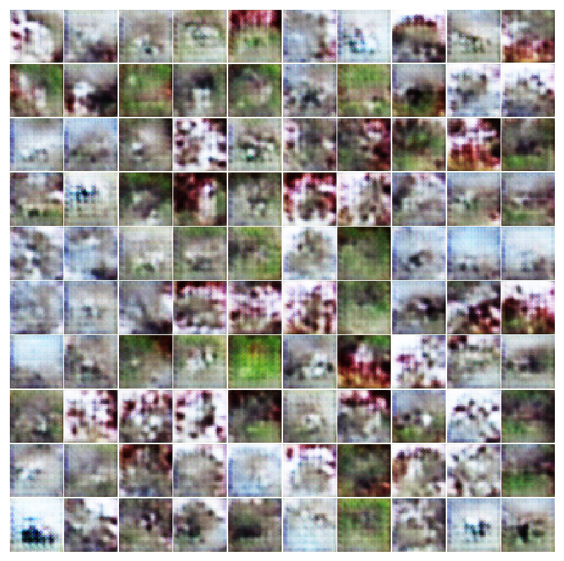 epoch 0
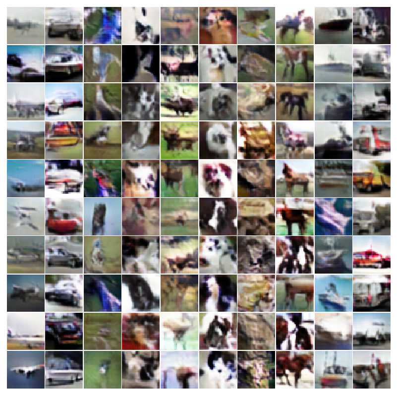 epoch 20
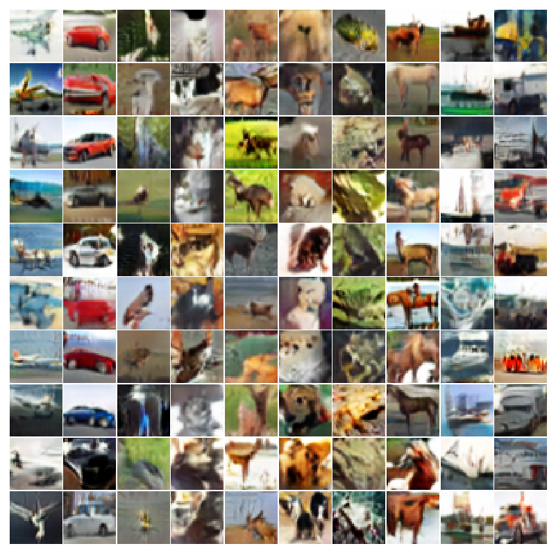 epoch 80
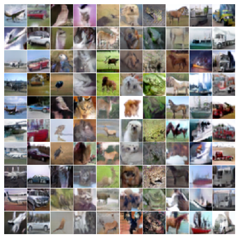 epoch 200
 final
final
Part 2 - Visualization
Perturb Real Images
This first part is following the technique mentioned in Tricking Networks
Use the same plot function from the previous section and load your discriminator model trained without the generator.
transform_test = transforms.Compose([
    transforms.CenterCrop(32),
    transforms.ToTensor(),
    transforms.Normalize((0.5, 0.5, 0.5), (0.5, 0.5, 0.5)),
])

testset = torchvision.datasets.CIFAR10(root='./', train=False, download=False, transform=transform_test)
testloader = torch.utils.data.DataLoader(testset, batch_size=batch_size, shuffle=False, num_workers=8)
testloader = enumerate(testloader)

model = torch.load('cifar10.model')
model.cuda()
model.eval()
batch_idx, (X_batch, Y_batch) = testloader.next()
X_batch = Variable(X_batch,requires_grad=True).cuda()
Y_batch_alternate = (Y_batch + 1)%10
Y_batch_alternate = Variable(Y_batch_alternate).cuda()
Y_batch = Variable(Y_batch).cuda()
Grab a sample batch from the test dataset. Create an alternative label which is simply +1 to the true label.
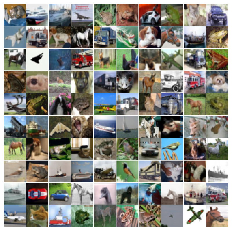
## save real images
samples = X_batch.data.cpu().numpy()
samples += 1.0
samples /= 2.0
samples = samples.transpose(0,2,3,1)

fig = plot(samples[0:100])
plt.savefig('visualization/real_images.png', bbox_inches='tight')
plt.close(fig)
Save the first 100 real images. Make sure to create the ‘visualization/’ directory beforehand.
_, output = model(X_batch)
prediction = output.data.max(1)[1] # first column has actual prob.
accuracy = ( float( prediction.eq(Y_batch.data).sum() ) /float(batch_size))*100.0
print(accuracy)
Get the output from the fc10 layer and report the classification accuracy.
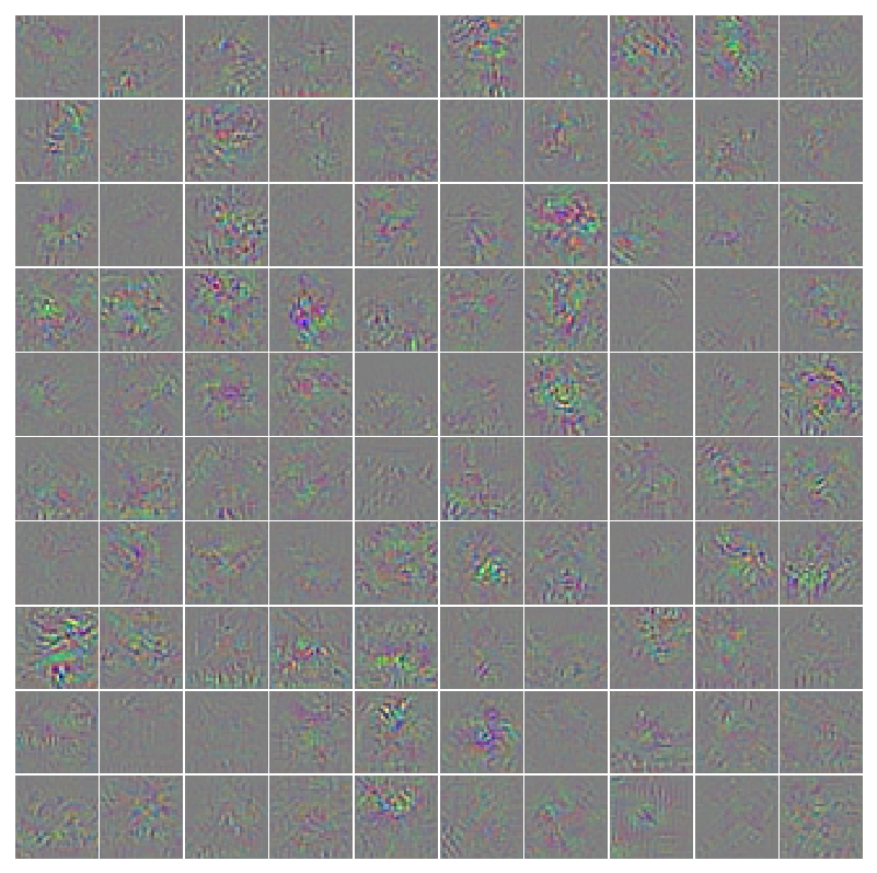
## slightly jitter all input images
criterion = nn.CrossEntropyLoss(reduce=False)
loss = criterion(output, Y_batch_alternate)

gradients = torch.autograd.grad(outputs=loss, inputs=X_batch,
                          grad_outputs=torch.ones(loss.size()).cuda(),
                          create_graph=True, retain_graph=False, only_inputs=True)[0]

# save gradient jitter
gradient_image = gradients.data.cpu().numpy()
gradient_image = (gradient_image - np.min(gradient_image))/(np.max(gradient_image)-np.min(gradient_image))
gradient_image = gradient_image.transpose(0,2,3,1)
fig = plot(gradient_image[0:100])
plt.savefig('visualization/gradient_image.png', bbox_inches='tight')
plt.close(fig)
Calculate the loss`` based on the alternative classes instead of the real classes.gradients``` is this loss backpropagated to the input image representing how a change in the input affects the change in the output class. Scale the gradient image between 0 and 1 and save it.
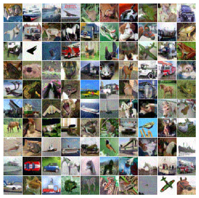
# jitter input image
gradients[gradients>0.0] = 1.0
gradients[gradients<0.0] = -1.0

gain = 8.0
X_batch_modified = X_batch - gain*0.007843137*gradients
X_batch_modified[X_batch_modified>1.0] = 1.0
X_batch_modified[X_batch_modified<-1.0] = -1.0

## evaluate new fake images
_, output = model(X_batch_modified)
prediction = output.data.max(1)[1] # first column has actual prob.
accuracy = ( float( prediction.eq(Y_batch.data).sum() ) /float(batch_size))*100.0
print(accuracy)

## save fake images
samples = X_batch_modified.data.cpu().numpy()
samples += 1.0
samples /= 2.0
samples = samples.transpose(0,2,3,1)

fig = plot(samples[0:100])
plt.savefig('visualization/jittered_images.png', bbox_inches='tight')
plt.close(fig)
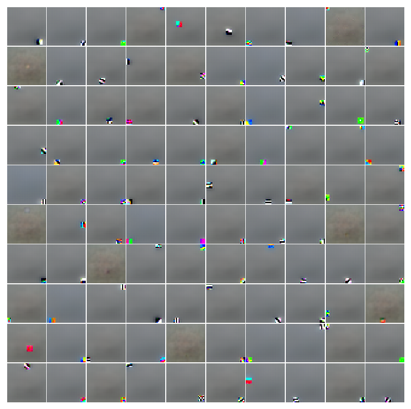
Modify the gradients to all be magnitude 1.0 or -1.0 and modify the original image. The example above changes each pixel by 10⁄255 based on the gradient sign. Evaluate these new image and also save it. You should end up with something similar to below with high accuracy reported on the real images and essentially random guessing for the altered images.
 real images
 gradients
 altered images
Synthetic Images Maximizing Classification Output
This section follows the technique described in section Feature Visualization. The loss function for each class will be used to repeatedly modify an image such that it maximizes
X = X_batch.mean(dim=0)
X = X.repeat(10,1,1,1)

Y = torch.arange(10).type(torch.int64)
Y = Variable(Y).cuda()
After loading in a model and a batch of images, calculate the mean image and make 10 copies (for the number of classes). Make a unique label for each copy.
lr = 0.1
weight_decay = 0.001
for i in xrange(200):
    _, output = model(X)

    loss = -output[torch.arange(10).type(torch.int64),torch.arange(10).type(torch.int64)]
    gradients = torch.autograd.grad(outputs=loss, inputs=X,
                              grad_outputs=torch.ones(loss.size()).cuda(),
                              create_graph=True, retain_graph=False, only_inputs=True)[0]

    prediction = output.data.max(1)[1] # first column has actual prob.
    accuracy = ( float( prediction.eq(Y.data).sum() ) /float(10.0))*100.0
    print(i,accuracy,-loss)

    X = X - lr*gradients.data - weight_decay*X.data*torch.abs(X.data)
    X[X>1.0] = 1.0
    X[X<-1.0] = -1.0

## save new images
samples = X.data.cpu().numpy()
samples += 1.0
samples /= 2.0
samples = samples.transpose(0,2,3,1)

fig = plot(samples)
plt.savefig('visualization/max_class.png', bbox_inches='tight')
plt.close(fig)
The model evaluates the images and extracts the output from the fc10 layer for each particular class. The gradient is calculated and the original image X is modified by this gradient in order to maximize the output. The learning rate, weight decay, and number of iterations can all be changed to produce different images. Perform this step with both models trained in part 1.
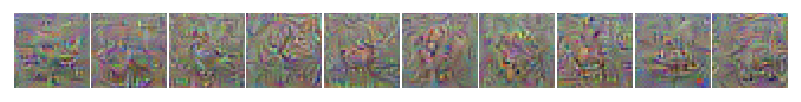 Synthetic images maximizing class output for discriminator trained without the generator
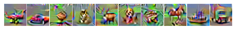 Synthetic images maximizing class output for discriminator trained with the generator
Synthetic Features Maximizing Features at Various Layers
You will need to modify the forward function of your discriminator before loading in the model.
def forward(self, x, extract_features=0):
Add an additional argument extract_features.
if(extract_features==8):
    h = F.max_pool2d(h,4,4)
    h = h.view(-1, no_of_hidden_units)
    return h
Within the forward function add the statement above after a convolution layer (in this particular case, after conv8). Make sure to perform max pooling (based on whatever dimensions the feature map from that particular layer has) and flatten the vector.
X = X_batch.mean(dim=0)
X = X.repeat(batch_size,1,1,1)

Y = torch.arange(batch_size).type(torch.int64)
Y = Variable(Y).cuda()

lr = 0.1
weight_decay = 0.001
for i in xrange(200):
    _, output = model(X)

    loss = -output[torch.arange(batch_size).type(torch.int64),torch.arange(batch_size).type(torch.int64)]
    gradients = torch.autograd.grad(outputs=loss, inputs=X,
                              grad_outputs=torch.ones(loss.size()).cuda(),
                              create_graph=True, retain_graph=False, only_inputs=True)[0]

    prediction = output.data.max(1)[1] # first column has actual prob.
    accuracy = ( float( prediction.eq(Y.data).sum() ) /float(batch_size))*100.0
    print(i,accuracy,-loss)

    X = X - lr*gradients.data - weight_decay*X.data*torch.abs(X.data)
    X[X>1.0] = 1.0
    X[X<-1.0] = -1.0

## save new images
samples = X.data.cpu().numpy()
samples += 1.0
samples /= 2.0
samples = samples.transpose(0,2,3,1)

fig = plot(samples[0:100])
plt.savefig('visualization/max_features.png', bbox_inches='tight')
plt.close(fig)
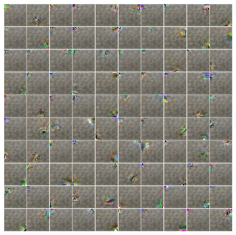
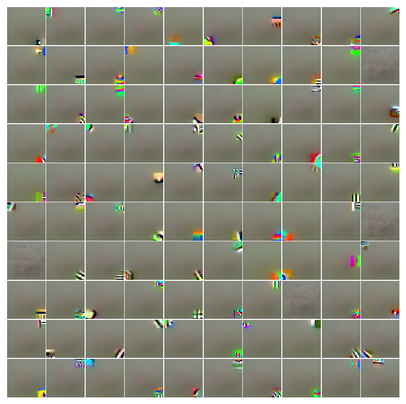
Similar to the section above, this will create synthetic images maximizing a particular feature instead of a particular class. You should notice the size of the feature gets larger for features later in the network. Posted below are some examples.
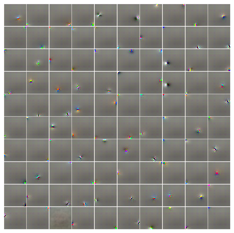 Synthetic images maximizing layer 2 features for discriminator trained without the generator
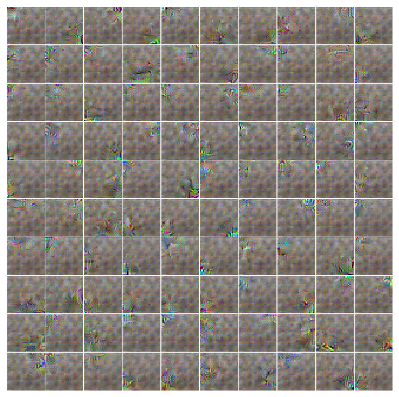
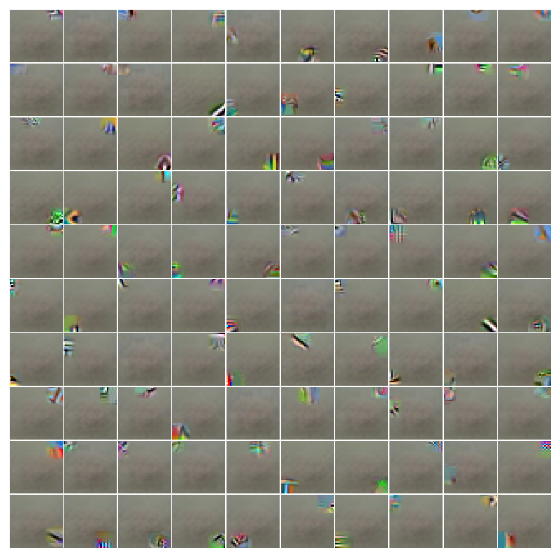
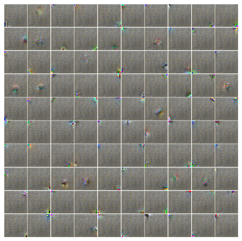 Synthetic images maximizing layer 3 features for discriminator trained without the generator
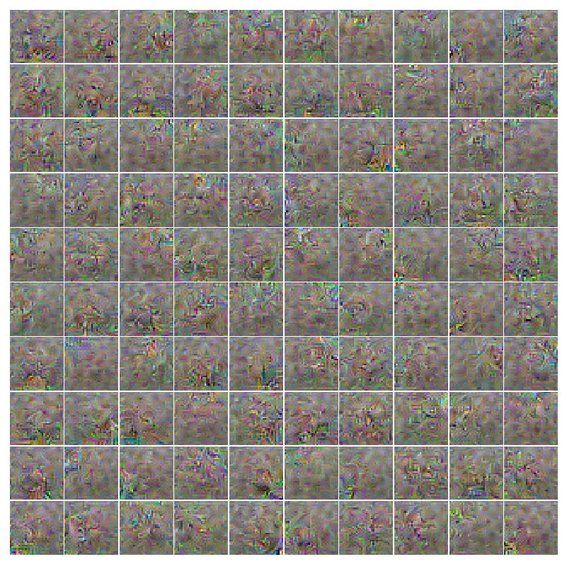
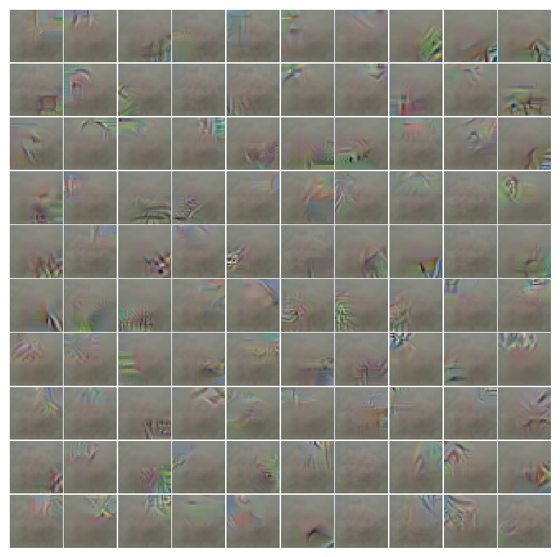
 Synthetic images maximizing layer 4 features for discriminator trained without the generator
 Synthetic images maximizing layer 6 features for discriminator trained without the generator
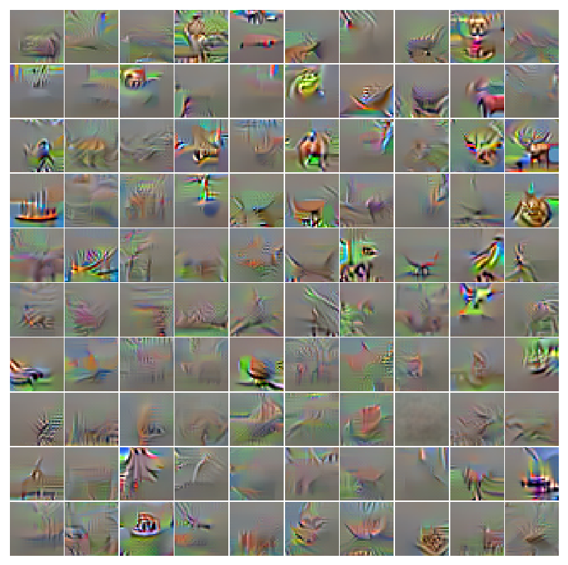
 Synthetic images maximizing layer 8 features for discriminator trained without the generator
 Synthetic images maximizing layer 2 features for discriminator trained with the generator
 Synthetic images maximizing layer 3 features for discriminator trained with the generator
 Synthetic images maximizing layer 4 features for discriminator trained with the generator
 Synthetic images maximizing layer 6 features for discriminator trained with the generator
 Synthetic images maximizing layer 8 features for discriminator trained with the generator
Results and what to turn in
At this point, hopefully you understand a little bit more about how CNNs work and how to implement a GAN.
You will submit your code along with a pdf document containing a few things.
- Choose 5-6 pictures of generated images to show how training progresses (for example - epoch 0, 100, 200, 300, 400, 500)
- From this part. A batch of real images, a batch of the gradients from an alternate class for these images, and the modified images the discriminator incorrectly classifies.
- From this part. Synthetic images maximizing the class output. One for the discriminator trained without the generator and one for the discriminator trained with the generator.
- From this part. Synthetic images maximizing a particular layer of features. Do this for at least two different layers (for example - layer 4 and layer 8.)
- Report your test accuracy for the two discriminators.
The classification performance is most likely slightly worse when the discriminator is trainined with a generator. There are papers that focus more on improving classification accuracy with GANs as opposed to generating realistic looking samples. It seems that it is possible to increase performance but the samples look worse with these techniques. It just depends on what you’re trying to achieve. For this assignment, I just wanted you to generate realistic looking images. Similarly, although the features seem to be more interpretable for the discriminator trained with the generator, that does not inherently mean they are in some way “better”. GANs are a new area of research, and there are lot of papers out there discussing this exact thing.