Overview

Release Date: 09/21/17

Due Date: 10/19/17

In this assignment you will:

• Learn to formulate and solve an optimization problem in the primal and dual spaces.
• Learn to use a markov random field for image denoising.
• Learn to train a deep convolutional auro-encoder for image denoising.
• Learn to train a deep structured model (deep convolutional auro-encoder + Markov Random Field) for image denoising

Written Section

Note: Answers without sufficient justification will not recieve any points.

Exercise 1:

1. Formulate the following problem as a linear optimization problem (i.e. both the objective and the constraints are linear):
   Minimize $\| Ax -B \|_{\infty}$

   with $A \in \mathbb{R}^{m \times n}$ and $B \in \mathbb{R}^{m}$.

2. Consider the optimization problem:

   Minimize $x^{2}+1$

   subject to $(x-2)(x-4) \leq 0$

   1. Analysis of primal problem. Give the feasible set, the optimal value, and the optimal solution.
   2. Lagrangian and dual function. Plot the objective $x^{2}+1$ versus $x$ . Show the feasible set, optimal point and its value, and plot the Lagrangian $L(x, \lambda)$ versus $x$ for a few positive values of $\lambda$.
   3. State the dual problem, and verify that it is a concave maximization problem. Find the dual optimal value and dual optimal solution $\lambda^{*}$. Does strong duality hold?

Exercise 2:

Consider the image $I$ presented by a rectangular grid of pixels. Given a noisy image $\hat{I}$, we want to recover the original image $I$ assumed to be smooth.

1. Write down the general form of a probability distribution over a MRF expressed in terms of an energy function $E$ and clique potentials $\Psi_{c}$.
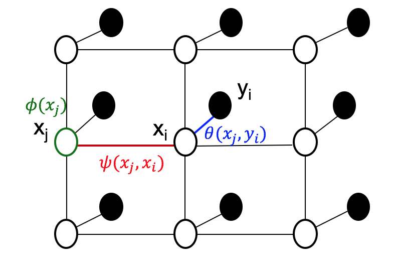
2. Let each pixel from the noisy image be a node in a graph $G$ with four connected neighbours, as it is shown in the figure below. $\{x_{i}\}$ are unobserved variables corresponding to the pixels of the unknown noise free image $I$. $\{y_{i}\}$ correspond to the pixels of the observed noisy image. The functions $\phi$, $\theta$ and $\psi$ correspond respectively to unary, observed-unobserved and unobserved-unobserved pairwise potentials. Write down the energy function corresponding to the MRF defined over $G$. What is the impact of the unary and pairwise potentials?
3. Write down the Energy function for the case of linear unary potentials and quadratic pairwise potentials: $\phi(x_{j})= a \cdot x_{j}, \psi(x_{i},x_{j})= - b \cdot x_{i} \cdot x_{j}$ and $\theta(x_{j},y_{j})= - c \cdot x_{j} \cdot y_{j}$, with a, b and c being positive real numbers. For this question, consider $x_{i},y_{i}\in\{-1,1\}$. Which configuration in general results in a minimum energy? (No calculations are required)
4. Formulate the image denoising task as an inference problem.
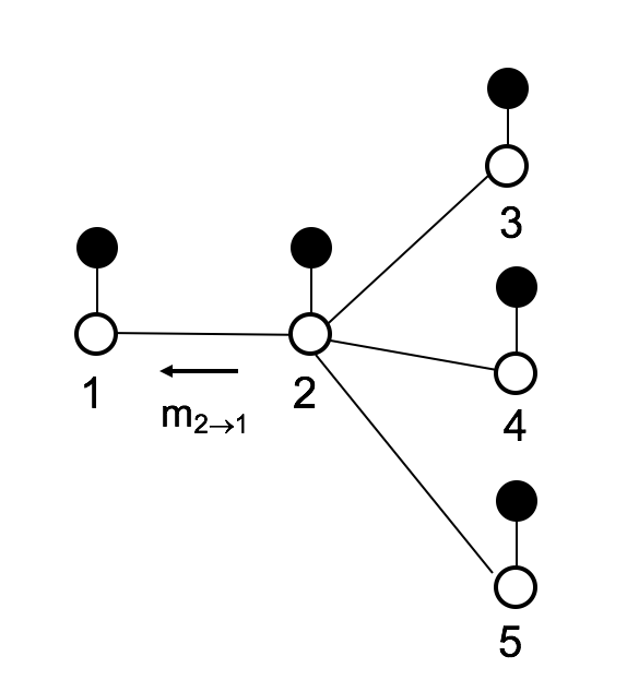
5. Using the belief propagation algorithm, compute the belief at node1 in the graph below (only consider the pairwise potentials).

---

Programming Section

Part 1: Setup

Follow the same steps as MP0 and MP1 to checkout and setup for MP2.

Part 2: Image Denoising with Markov Random Field

Similar to the setting of Exercise 2, from a noisy image $\hat{I}$, we want to recover an image $I$ that is both smooth and close to $\hat{I}$ by maximizing the probability of $I$ given $\hat{I}$. $P(I|\hat{I})$ is a distribution over a Markov Random Field, characterized by the following energy function:

$E(x,y)= - \alpha \sum\limits_{i,j\in N(i)} x_{i} \cdot x_{j} - \beta \sum\limits_{i} x_{i} \cdot y_{i}- \gamma \sum\limits_{i} x_{i}$ where $x_{i}\in \{-1,1\}$ are the hidden variables corresponding to the pixels of the noise-free image and $y_{i}$ are the observed variables corresponding to the pixels of the noisy image. $\alpha, \beta,$ and $\gamma$ are positive constants. $N(i)$ denotes the neighbouring pixels to $x_{i}$.

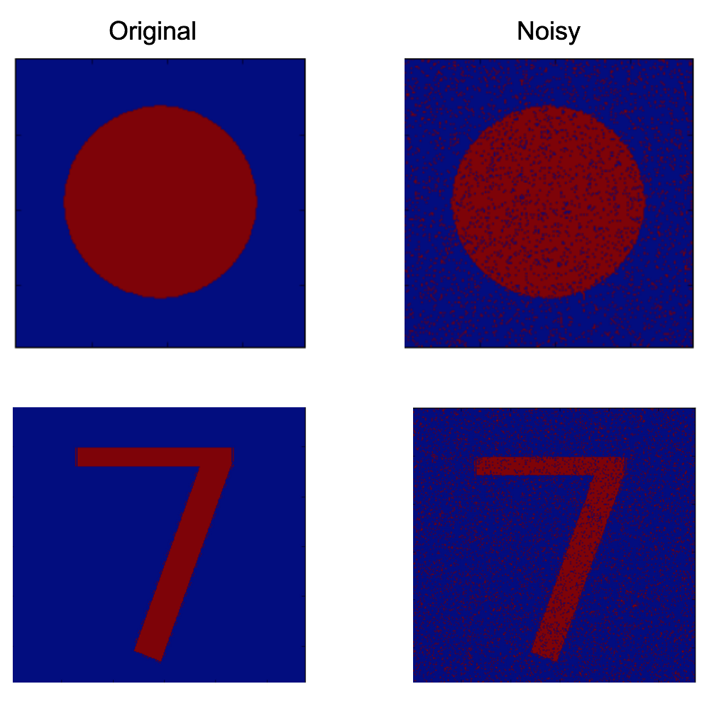
In this assignment, you will corrupt the images below with some random noise, then infer the noise-free version by minimizing the energy function above. In MRF.py, the overall program structure as well as the missing function interfaces with detailed required functionality are provided for you.

Part 3: Image Denoising with a Convolutional Auto-Encoder

For this part, you will perform image denoising using a denoising autoencoder. The model is fed with noisy images from the MNIST dataset and trained to reconstruct the original ones. The overall program structure is provided to you in DeepAE/train.py. Follow the following steps to build and train the model:

1. In DeepAE/utils.py, implement the function add_noise which corrupts a batch of images with random noise by flipping the value of a pixel to 0 or 1 with probability 0.1.
2. In DeepAE/model.py, implement the method build_inputs which defines three placesholders for respectively (1) noise-free images, (2) noisy images and (3) a boolean indicating whether the model is being trained or tested.
3. In DeepAE/model.py, implement the method build_model by designing an autoencoder model that takes as input the noisy images and returns reconstructed ones. Feel free to experiment with different architectures. Explore the effect of 1) fully connected layers, 2) convolution layers, 3) interlayer batch normalization, 7) dropout, downsampling methods(strided convolution vs max-pooling) 8) upsampling methods (upsampling vs deconvolution), 9) different optimization methods (e.g., stochastic gradient descent versus stochastic gradient descent with momentum versus RMSprop. Do not forget to scale the final output between 0 and 1.

4. Run train.sh to train the model. Run evaluate.sh in a separate process for the periodic evaluation. Our solution has a loss of 0.09 after 3000 iterations. We expect your solution to be in the same range.

Part 6: Submit

Submitting your code is simply commiting you code. This can be done with the follow command:

svn commit -m "Some meaningful comment here."

Note The assignment will be autograded. It is important that you do not use additional libraries, or change the provided functions input and output.