ECE 486 Control Systems
Lecture 15
Stability in Terms of Frequency Response
Last time, we discussed how to sketch Bode plots using Bode form. This form can be seen as the product of three basic types of factors.
In this lecture, we shall further study the relationship between stability and frequency response. In the process of doing so, we shall introduce gain margin and phase margin. At the end of this lecture, we shall be able to read off stability properties of the closed loop system from the Bode plot of the open loop transfer function. Given gain and phase margins, we shall have rough ideas of our “distance to” instability.
Consider this unity feedback configuration

Figure 1: Unity feedback with open loop \(KG(s)\)
It is a natural question that how we decide whether the closed loop system is stable for a given value of \(K > 0\) based on our knowledge of the open loop transfer function \(KG(s)\). Well, we did answer this question through Lecture 10 and Lecture 11 using Root Locus method.
Indeed, points on the root locus satisfy the characteristic equation
\begin{align*} 1 + KG(s) = 0 &\iff KG(s) = -1 \\ &\iff G(s) = - \frac{1}{K}. \end{align*}If \(s \in \CC\) is on the root locus, then by matching the magnitude and phase of \(-1\), we have
\begin{align*} \left| KG(s) \right| = 1 \, \text{ and } \,\angle KG(s) = \angle G(s) = 180^\circ \bmod 360^\circ. \end{align*}Another approach is we can use its Bode plots. Indeed,
\begin{align*} \omega &\longmapsto |KG(j\omega)| \qquad \hspace{1mm} \text{on log-log scale} \\ \omega &\longmapsto \angle KG(j\omega) \qquad \text{on log-linear scale} \end{align*}Bode plots show us magnitude and phase, but only for an open loop transfer function \(KG(s)\) evaluated at \(s=j\omega\), \(0 < \omega < \infty\), whereas the root locus, using some open loop \(L(s)\), shows the complex trajectory of closed loop poles when ranging some parameter \(K \in (0, +\infty)\).
We already know from Routh-Hurwitz criterion and root locus technique that when closed loop poles move across imaginary axis, the closed loop system stability goes from stability to instability and vice versa. In order to establish the relationship between this transition and Bode plot, consider some $jω$-crossings on the root locus. If some \(s=j\omega\) is on the root locus for some value of \(K\), then
\begin{align*} \left| KG(j\omega) \right| = 1 \, \text{ and } \, \angle KG(j\omega) = 180^\circ \bmod 360^\circ. \end{align*}Therefore, the transition from stability to instability can be detected in two different ways
- from root locus, find the $jω$-crossings;
- from Bode plots, find the frequency where \(M=1\) and \(\phi = 180^\circ\) for a given value of \(K\).
Example 1: Consider the following open loop transfer function
\begin{align*} KG(s) = \frac{K}{s (s^2 + 2s + 2)}. \end{align*}We try to find the critical \(K\) that gives $jω$-crossings on root locus plot and further find the frequency \(\omega\) where magnitude and phase of \(KG(j\omega)\) correspond to the found $jω$-crossings.
Solution: By the given \(KG(s)\) above, its associated characteristic equation is given by
\begin{align*} 1 + \frac{K}{s (s^2 + 2s + 2)} &= 0 \\ \implies s (s^2 + 2s + 2) + K &= 0 \\ s^3 + 2s^2 + 2s + K &= 0. \end{align*}Recall the necessary and sufficient condition for stability for a third degree polynomial \(s^3 + a_1 s^2 + a_2 s + a_3\),
\begin{align*} a_1,a_2,a_3 > 0 \, &\text{ and } \, a_1 a_2 > a_3 \\ \implies K > 0 \, &\text{ and } \, 2\times 2 > K. \end{align*}The closed-loop system is stable if and only if \(0 < K < 4\).
Let’s see what we can read off from the Bode plots. Rewrite \(KG(s)\) in Bode form
\begin{align*} KG(j\omega) = \frac{K}{2 j\omega \left(\big(\frac{j\omega}{\sqrt{2}}\big)^2 + j\omega + 1 \right)}. \end{align*}Plot the magnitude first,
- Type \(1\) factor \(\dfrac{\frac{K}2}{j\omega}\) has \(K_0 = \frac{K}2\) and \(n = -1\), therefore its low frequency asymptote is a line with slope \(-1\) passing through \((\omega, M)=(1,\frac{K}2)\).
- Type \(3\) factor with complex poles has breakpoint at \(\omega = \sqrt{2}\). At that breakpoint frequency, it steps slope down by \(2\).
- The damping \(\zeta = \dfrac{1}{\sqrt{2}}\), therefore there is no reasonant peak.
With \(K_{\rm critical} = 4\), the magnitude plot of
\begin{align*} KG(j\omega) = \frac{K}{2 j\omega \left(\big(\frac{j\omega}{\sqrt{2}}\big)^2 + j\omega + 1 \right)} \end{align*}is shown in Figure 2.
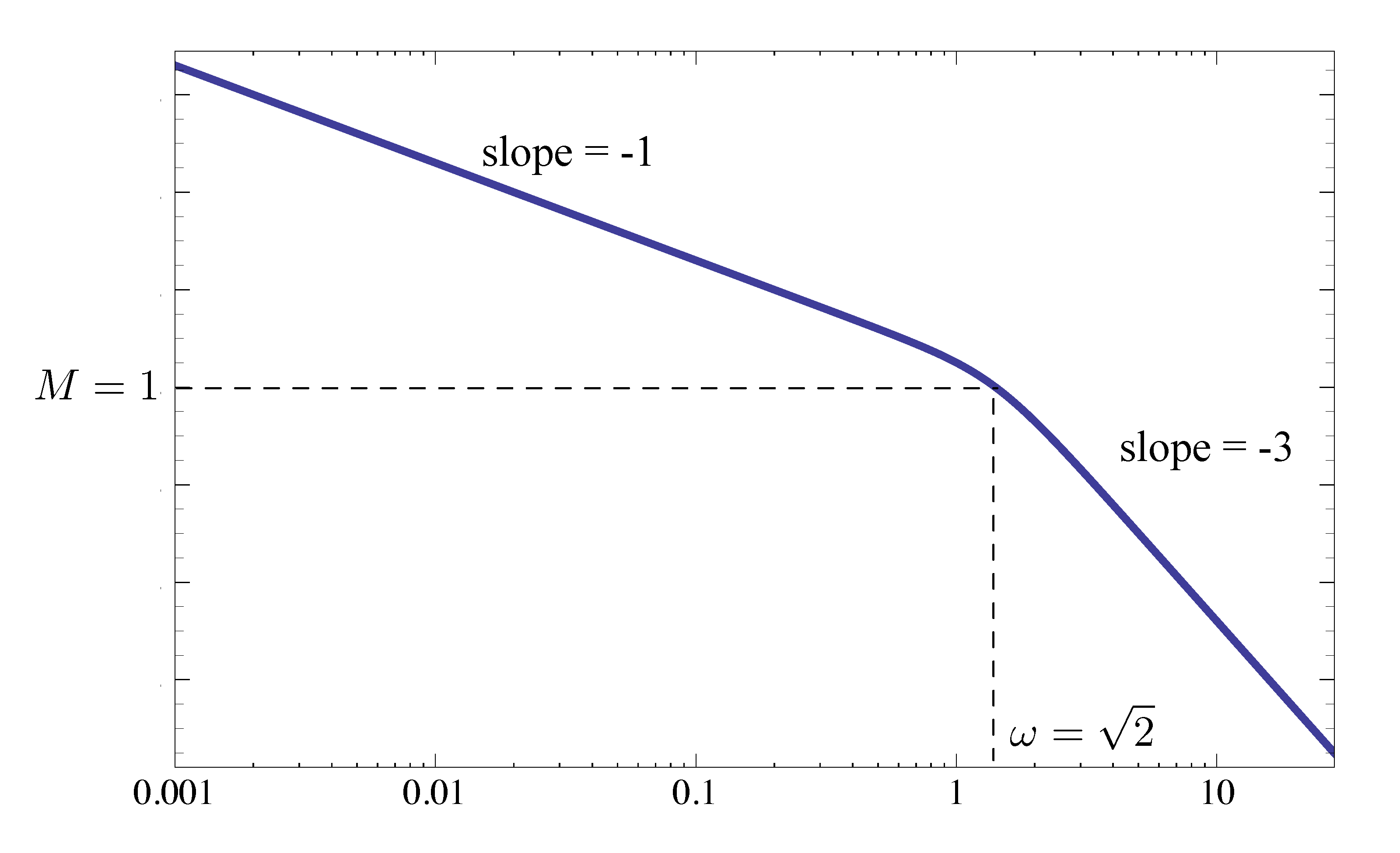
Figure 2: Example 1, magnitude plot with \(K_{\rm critical} = 4\)
Further we note when \(\omega = \sqrt{2}\), the magnitude
\begin{align*} M &= \left| 4G(j\omega)\right| \\ &= \left| \dfrac{2}{j\sqrt{2} \left( j^2 + j\sqrt{2} + 1\right)}\right| \\ &= 1. \end{align*}Next we plot the phase of \(KG(s)\). In this case it is independent of \(K\).
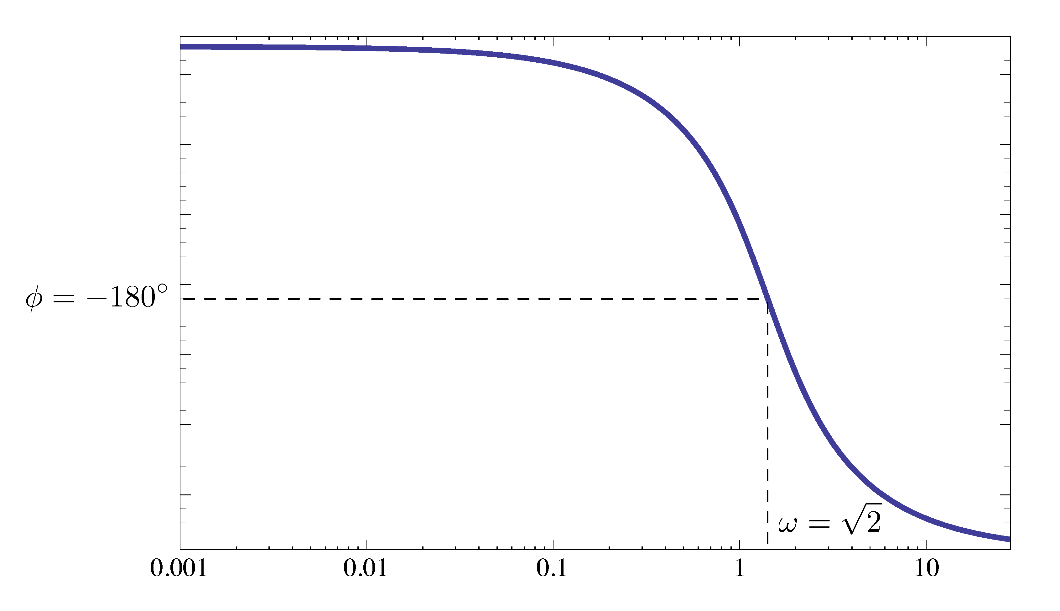
Figure 3: Example 1, phase plot with \(K_{\rm critical} = 4\)
We note when \(\omega = \sqrt{2}\), \(\phi = -180^\circ\).
In conclusion, for the critical value \(K=4\), we have magnitude \(M=1\) and phase \(\phi = 180^\circ \bmod 360^\circ\) at \(\omega = \sqrt{2}\).
Crossover Frequency and Stability
From Example 1 above, it seems the transitioning between stability and instability, i.e., $jω$-crossings are related to magnitude \(1\) and phase \(-180^\circ\).
Indeed, the frequency at which \(M=1\) is called the crossover frequency and denoted by \(\omega_c\). Using the magnitude from Example, we see

Figure 4: Crossover frequency is \(\omega_c = \sqrt{2}\) in Example 1
When transitioning from stability to instability, on the Bode plot (phase plot)
\begin{align*} \angle KG(j\omega_c) = -180^\circ \end{align*}for some critical \(K\).
Effect of Varying \(K\)
When \(K\) (here a scalar, not to be confused with a controller block \(K(s)\)) is changing, although \(K\) will not contribute to phase, it moves around the crossover frequency \(\omega_c\). Indeed, for example,
if we multiply \(K\) by \(2\),
\begin{align*} \log (2M) &= \log 2 + \log M. \end{align*}Then the magnitude plot shifts up by \(\log 2\);
if we divide \(K\) by \(2\),
\begin{align*} \log \left(\dfrac{1}{2}M \right) &= \log \dfrac{1}{2} + \log M \\ &= -\log 2 + \log M. \end{align*}Then the magnitude plot shifts down by \(\log 2\).
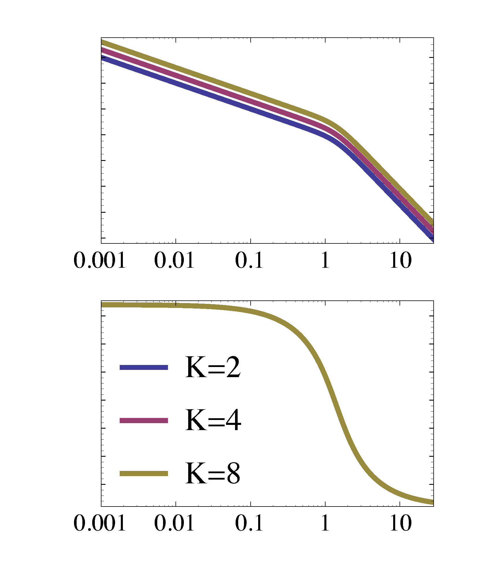
Figure 5: Crossover frequency is moved around by changing \(K\) but phase stays the same
Therefore, as for Example 1, we have
\begin{align*} \angle KG(j\omega_c) \begin{cases} > - 180^\circ, & \text{for $K < 4$} & \text{ (stable)} \\ = -180^\circ, & \text{for $K=4$} & \text{ (critical)} \\ < - 180^\circ, & \text{for $K > 4$} & \text{ (unstable)} \end{cases} \end{align*}Equivalently, we may define \(\omega_{180^\circ}\) as the frequency at which
\[ \phi = 180^\circ \bmod 360^\circ. \]
Then, in Example 1,
\begin{align*} \left| KG(j\omega_{180^\circ})\right| < 1 & \iff \text{stability} \\ \left| KG(j\omega_{180^\circ})\right| > 1 & \iff \text{instability} \end{align*}Important: The above equivalence is not a general rule; conditions may vary depending on the system. Sometimes, we must use either root locus or Nyquist plot to resolve ambiguity. Nevertheless, it is the motivation for us to introduce gain margin and phase margin below.
Gain Margin
Our next natural question would be
Question: Can we use the Bode plot to determine how far from instability we are?
To answer this question, we shall introduce two important characteristics gain margin (GM) and phase margin (PM).
We define gain margin (GM) as the factor by which \(K\) can be multiplied before we get \(M=1\) when \(\phi = 180^\circ\).
Since varying \(K\) does not change \(\omega_{180^\circ}\), to find gain margin we need to inspect magnitude \(M\) at \(\omega=\omega_{180^\circ}\).
Recall Example 1 where \(G(s) = \frac{1}{s(s^2 + 2s + 2)}\), when \(K=2\) (stable), the margin in magnitude plot is shown in Figure 6.
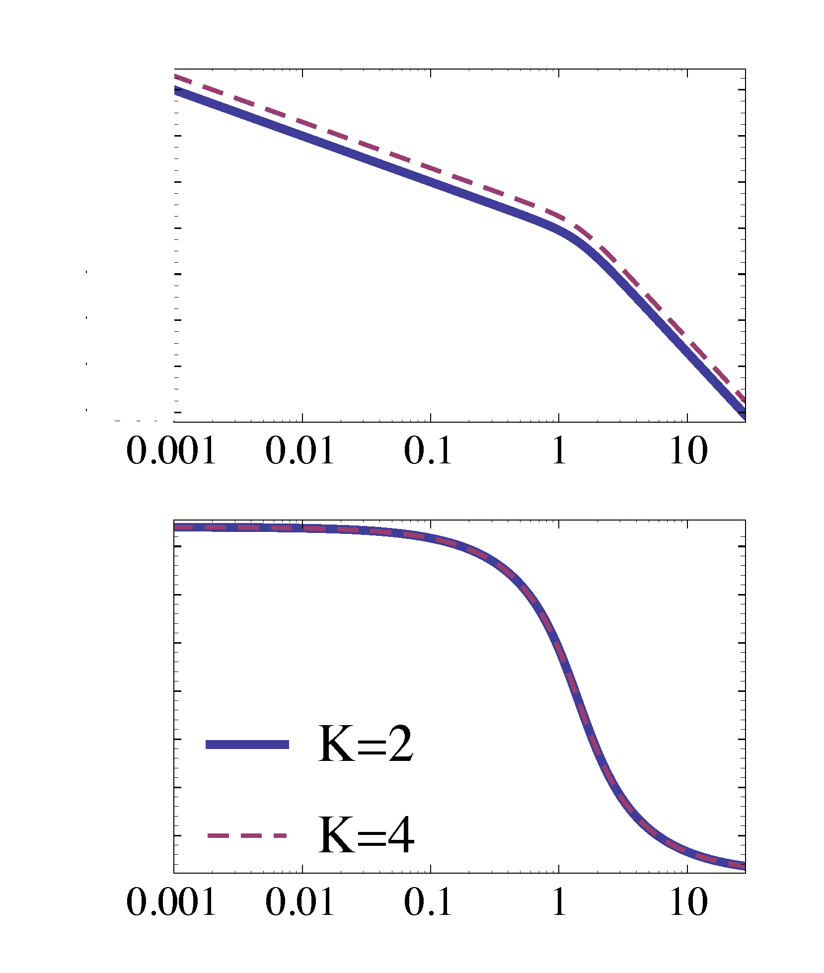
Figure 6: Margin in magnitude plot when \(K = 2\) in Example 1
To compute the gain margin, from Figure 7,
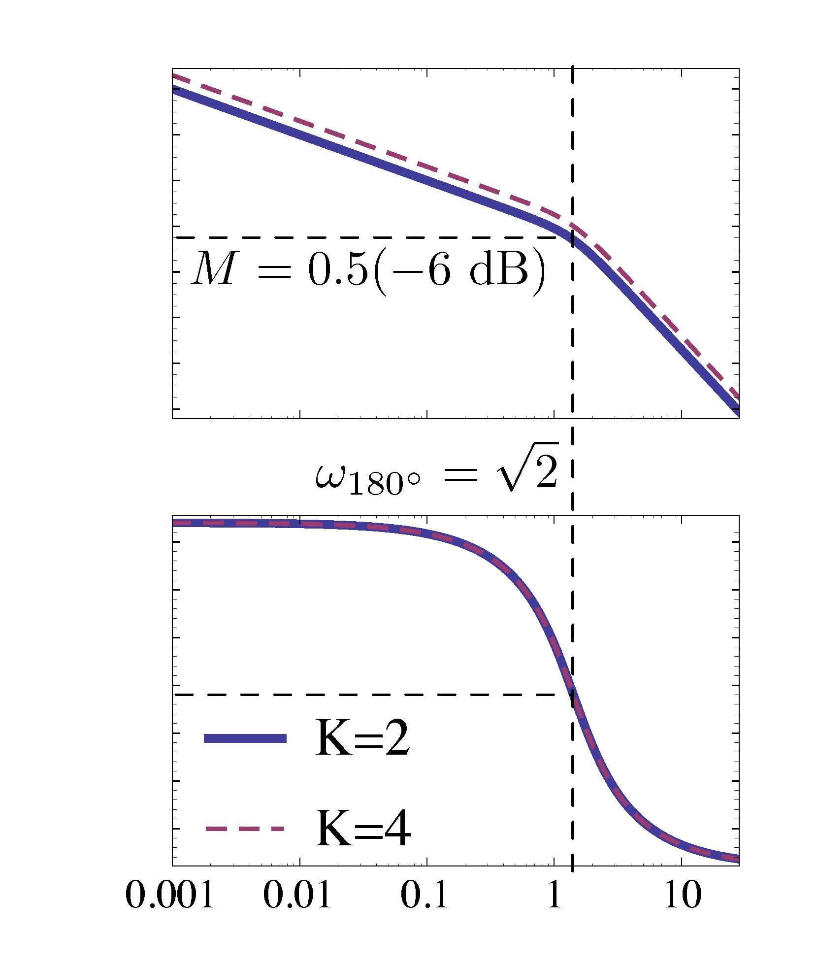
Figure 7: Compute gain margin when \(K = 2\) in Example 1
\(\omega_{180^\circ} = \sqrt{2}\), at this frequency, the magnitude \(M = 0.5\) or $-6$dB. Therefore, The gain margin in this case is \(2\).
Phase Margin
We shall continue to use
\[ G(s) = \dfrac{1}{s(s^2 + 2s + 2)} \]
when \(K=2\) (stable) to illustrate the discussion of phase margin.
We define phase margin (PM) as the amount by which the phase at the crossover frequency \(\omega_c\) differs from \(180^\circ \bmod 360^\circ\).
To find PM, we need to inspect \(\phi\) at \(\omega = \omega_c\).
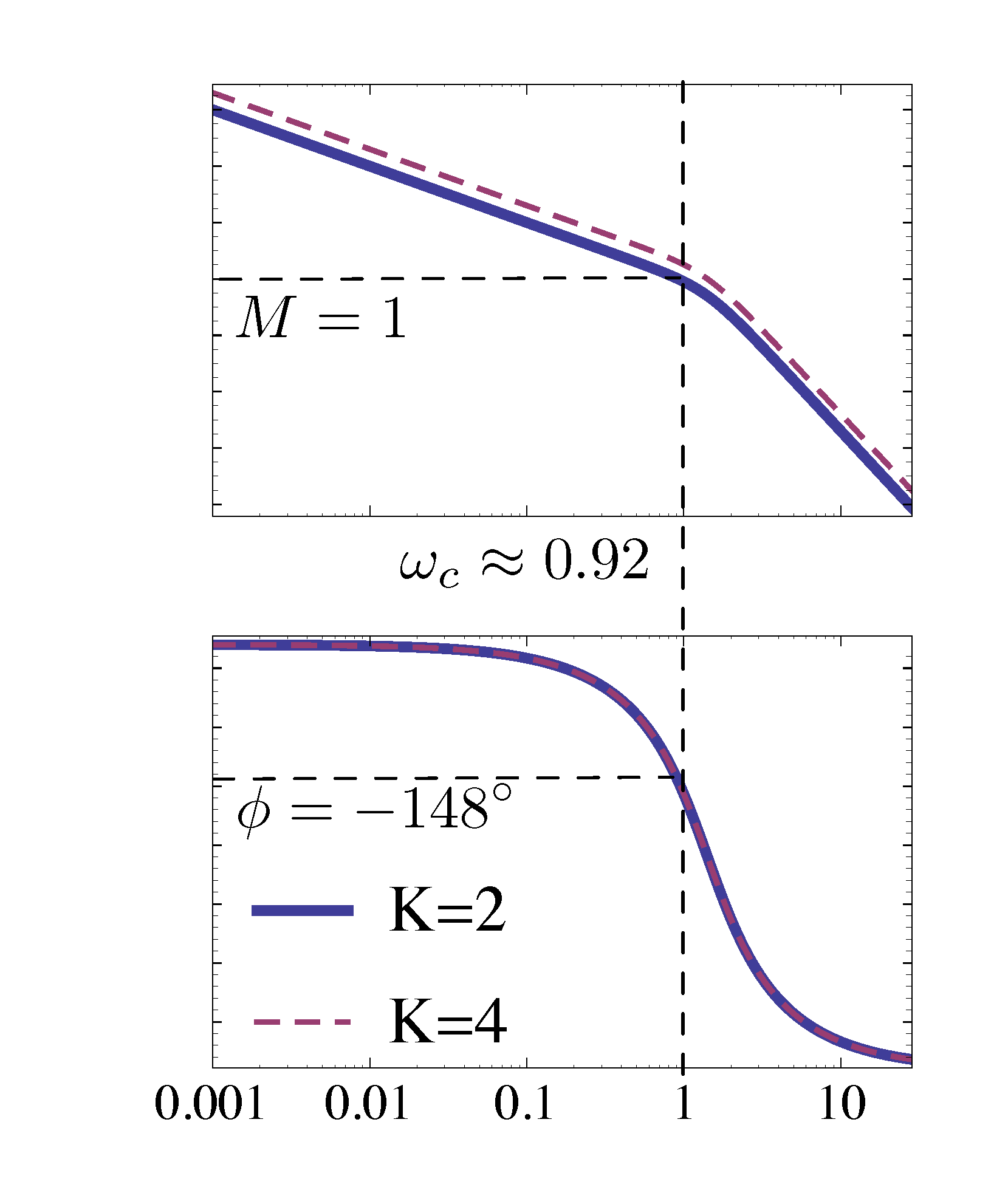
Figure 8: Compute phase margin when \(K = 2\) in Example 1
In Example 1, at crossover frequency \(\omega_c \approx 0.92\), phase \(\phi = -148^\circ\). Therefore, phase margin is \((-148^\circ) - (-180^\circ) = 32^\circ\). In many practical applications, we may want phase margin to be \(\text{PM} \ge 30^\circ\).
Example 2: Consider unity feedback configuration as in Figure 9,

Figure 9: Example 2 with unity feedback
where
\[ G(s) = \frac{\omega^2_n}{s^2 + 2\zeta\omega_n s}, \, \text{ with } \zeta,\omega_n > 0. \]
Investigate the gain margin and phase margin when \(K = 1\).
Solution: Consider gain \(K=1\). It follows that the closed loop transfer function
\begin{align*} \frac{KG(s)}{1+KG(s)} &= \frac{\dfrac{\omega^2_n}{s^2 + 2\zeta\omega_n s}}{1 + \dfrac{\omega^2_n}{s^2 + 2\zeta\omega_n s}} \\ &= \frac{\omega^2_n}{s^2 + 2\zeta\omega_n s + \omega^2_n}. \end{align*}This gives the prototype second order transfer function.
We will show \(\text{GM} = \infty\). Indeed
\begin{align*} G(j\omega) &= \frac{\omega^2_n}{(j\omega)^2 + 2\zeta\omega_n j\omega} \\ &= \frac{\omega_n}{2\zeta j\omega \left(\frac{j\omega}{2\zeta\omega_n} + 1\right)}. \tag{1} \label{d15_eq1} \end{align*}The phase plot is given by Figure 10.
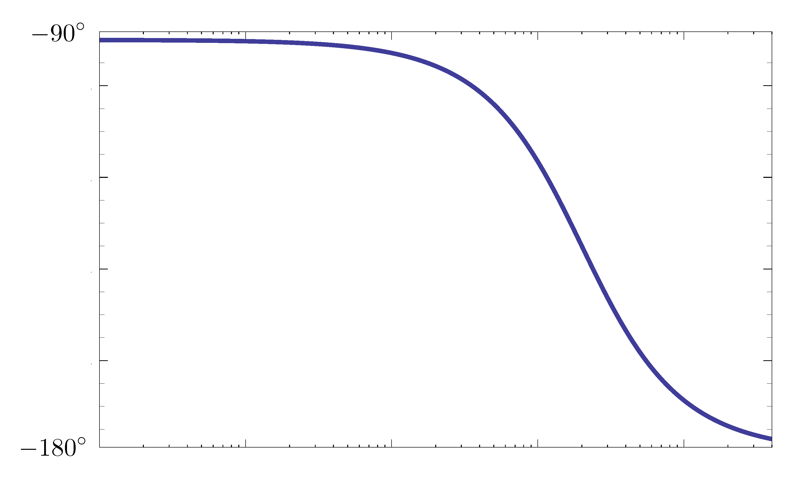
Figure 10: Example 2 Bode plot — phase plot
We notice
- the phase plot starts at \(-90^\circ\) (Type 1 factor with \(n=-1\))
- the phase plot goes down by \(-90^\circ\) (Type 2 factor of a pole)
Recall to find gain margin, we first need to find \(\omega_{180^\circ}\). But here there is no such an \(\omega\), i.e., no gain margin can be computed. We say the gain margin is infinity in this case.
It means that we can keep on increasing \(K\) indefinitely without ever encountering instability.
It confirms what we already knew — the characteristic polynomial of prototype second order transfer function is
\[ p(s) = s^2 + 2\zeta\omega_n s + \omega^2_n, \]
which is always stable for given \(\zeta\) and \(\omega_n\).
To compute the phase margin, we need to generate the magnitude plot. By \(KG(j\omega) = G(j\omega)\) in Equation \eqref{d15_eq1}
- Type 1 factor with \(n = -1\) gives a low frequency asymptote with slope \(-1\).
- Type 2 factor makes slope step down by \(1\) past the breakpoint \(\omega = 2\zeta\omega_n\).
The magnitude plot crosses $0$db line or \(M = 1\) so there is a finite crossover frequency \(\omega_c\) as shown in Figure 11.
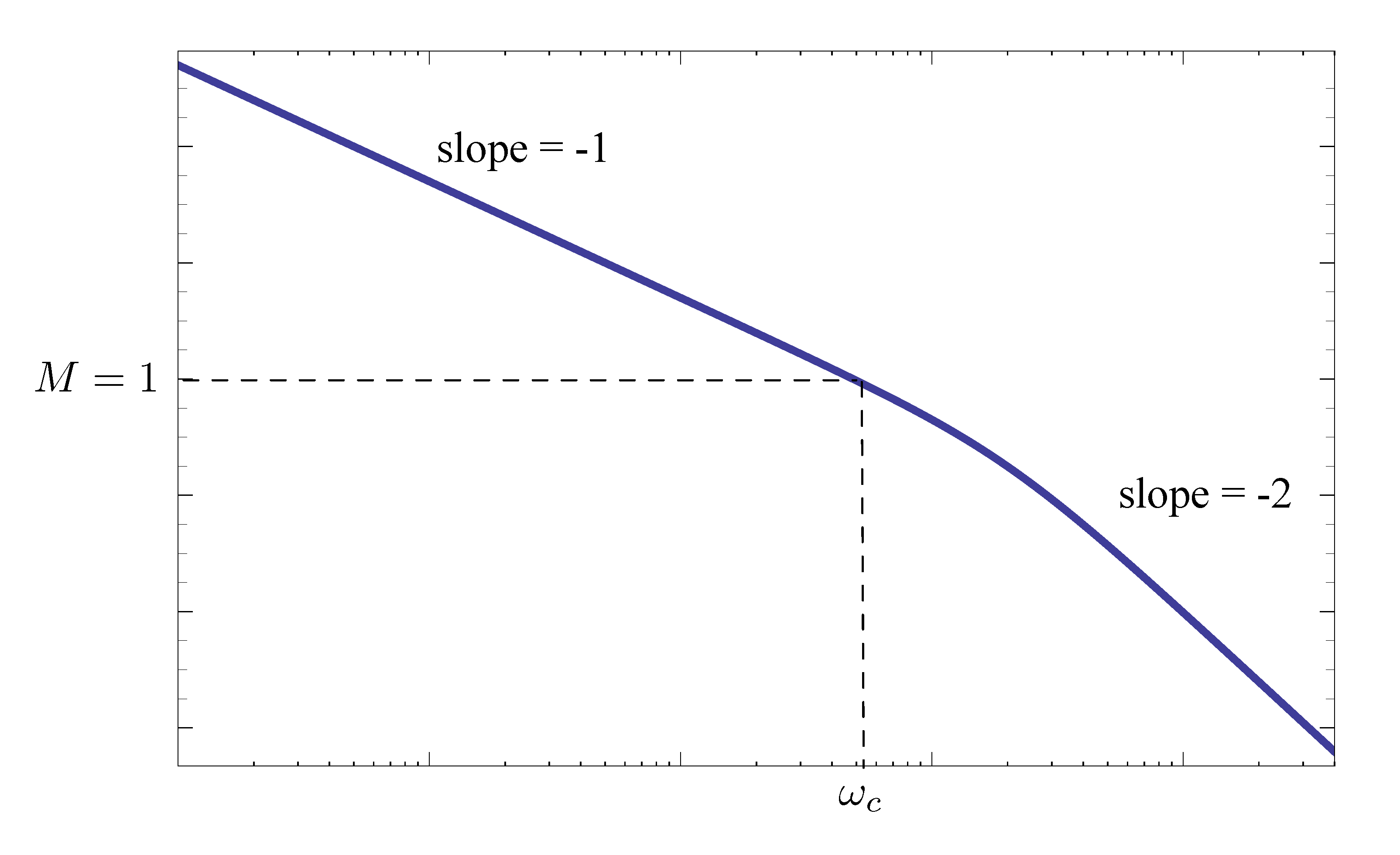
Figure 11: Example 2 Bode plot — magnitude plot
It can be shown that for system in this example
\[ \text{PM}\Big|_{K=1} = \tan^{-1}\left( \frac{2\zeta}{\sqrt{\sqrt{4\zeta^4+1}-2\zeta^2}} \right). \]
A useful approximation for \(\text{PM} < 70^\circ\) is that we can use \(\text{PM} \approx 100 \zeta\).
We can deduce from Example 2 above that for a second order system, by
\[ \text{PM}\Big|_{K=1} = \tan^{-1}\left( \frac{2\zeta}{\sqrt{\sqrt{4\zeta^4+1}-2\zeta^2}} \right) \approx 100 \zeta, \]
larger phase margin means larger (better) damping. Hence we can relate a closed loop characteristic damping ratio to an open-loop quantity phase margin.
Thus, the overshoot \(M_p = \exp\left( - \frac{\pi\zeta}{\sqrt{1-\zeta^2}}\right)\) and resonant peak \(M_r = \frac{1}{2\zeta\sqrt{1-\zeta^2}}-1\) are both related to phase margin through \(\zeta\).
Bode’s Gain-Phase Relationship
In the next lecture, we will see the following more generally. Bode’s Gain-Phase Relationship states all important characteristics of the closed loop time response can be related to the phase margin of the open loop transfer function.
In fact, we will use a quantitative statement of this relationship as a design guideline.