CS440/ECE448 Fall 2018

Assignment 4: Reinforcement Learning and Deep Learning

Deadline: Tuesday, May 1, 11:59:59PM

Contents

• Part 1: Q-learning (Pong)
  • Setup for Single-Player Pong
  • Part 1.1 (for everybody): Single-Player Pong
  • Part 1.2 (for 4-credit students): Environment Changed
  • Part 1 Extra Credit
• Part 2: Deep Learning (Pong)
  • Part 2.1 (for everybody): Cloning the Behavior of an Expert Player
  • Part 2.2 (for 4-credit students): Deep Q-Learning
  • Part 2 Extra Credit
• Report Checklist
• Submission Instructions

Part 1: Q-Learning (Pong)

Created by Daniel Calzada and redesigned by Peixin Chang

In 1972, the game of Pong was released by Atari. Despite its simplicity, it was a ground-breaking game in its day, and it has been credited as having helped launch the video game industry. In this assignment, you will create a simple version of Pong and use Q-learning (TD-learning) and SARSA to train agents to play the game.

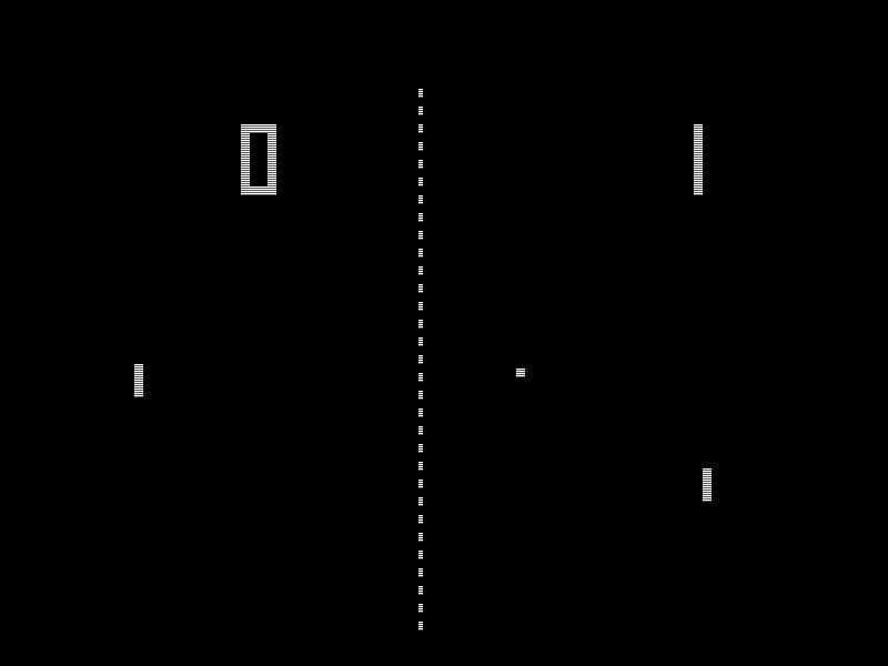
Image from Wikipedia

Environment for Single-Player Pong (for everybody)

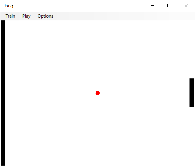
Single-player Pong

Instructions for Part 1 and Part 2: Before implementing the algorithms, we must first create the environment for a single-player version of Pong. Let's define the Markov Decision Process (MDP) as follows:

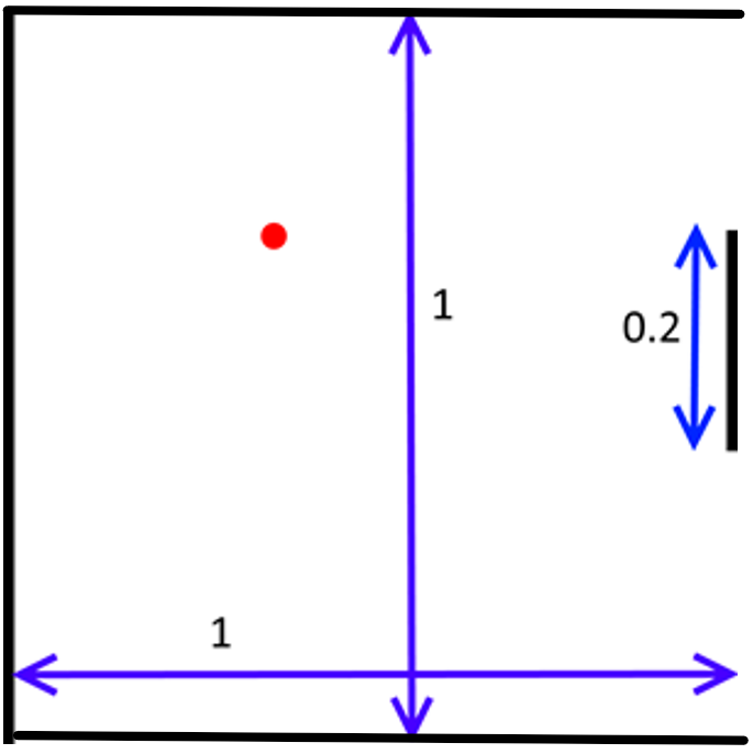
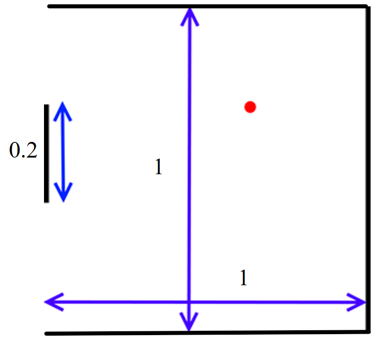
• State: A tuple (ball_x, ball_y, velocity_x, velocity_y, paddle_y).
  • ball_x and ball_y are real numbers on the interval [0,1]. The lines x=0, y=0, and y=1 are walls; the ball bounces off a wall whenever it hits. The line x=1 is defended by your paddle.
  • The absolute value of velocity_x is at least 0.03, which guarantees that the ball is moving either left or right at a reasonable speed.
  • paddle_y represents the top of the paddle (the side closer to y=0) and is on the interval [0, 1 - paddle_height], where paddle_height = 0.2, as can be seen in the image above. (The x-coordinate of the paddle is always paddle_x=1, so you do not need to include this variable as part of the state definition).
• Actions: Your agent's actions are chosen from the set {nothing, paddle_y += 0.04, paddle_y -= 0.04}. In other words, your agent can either move the paddle up, down, or make it stay in the same place. If the agent tries to move the paddle too high, so that the top goes off the screen, simply assign paddle_y = 0. Likewise, if the agent tries to move any part of the paddle off the bottom of the screen, assign paddle_y = 1 - paddle_height.
• Rewards: +1 when your action results in rebounding the ball with your paddle, -1 when the ball has passed your agent's paddle, or 0 otherwise.
• Initial State: Use (0.5, 0.5, 0.03, 0.01, 0.5 - paddle_height / 2) as your initial state (see the state representation above). This represents the ball starting in the center and moving towards your agent in a downward trajectory, where the agent's paddle starts in the middle of the screen.
• Termination: Consider a state terminal if the ball's x-coordinate is greater than that of your paddle, i.e., the ball has passed your paddle and is moving away from you.

We need to simulate the environment. The ball is a single point, and your paddle is a line. Therefore, you don't need to worry about the ball bouncing off the ends of the paddle. At each time step, you must:

• Update the paddle position based on the action chosen by your agent.
• Increment ball_x by velocity_x and ball_y by velocity_y.
• Bounce:
  • If ball_y < 0 (the ball is off the top of the screen), assign ball_y = -ball_y and velocity_y = -velocity_y.
  • If ball_y > 1 (the ball is off the bottom of the screen), let ball_y = 2 - ball_y and velocity_y = -velocity_y.
  • If ball_x < 0 (the ball is off the left edge of the screen), assign ball_x = -ball_x and velocity_x = -velocity_x.
  • If moving the ball to the new coordinates resulted in the ball bouncing off the paddle, handle the ball's bounce by assigning ball_x = 2 * paddle_x - ball_x. Furthermore, when the ball bounces off a paddle, randomize the velocities slightly by using the equation velocity_x = -velocity_x + U and velocity_y = velocity_y + V, where U is chosen uniformly on [-0.015, 0.015] and V is chosen uniformly on [-0.03, 0.03]. As specified above, make sure that all |velocity_x| > 0.03.
    
    Note: In rare circumstances, either of the velocities may increase above 1. In these cases, after applying the bounce equations given above, the ball may still be out of bounds. If this poses a problem for your implementation, feel free to impose the restriction that |velocity_x| < 1 and |velocity_y| < 1.

Instructions only for Part 1: Because this state space is continuous, to allow for it to be learned with Q-learning, we need to be able to convert the continuous state space into a discrete, finite state space. To do this, please follow the instructions below. Note that the constants may be different for the next part of the assignment, so it would be wise to define these as constants in a separate part of your code so you can change them easily. You will learn how to deal with continuous state spaces in part 2.

• Treat the entire board as a 12x12 grid, and let two states be considered the same if the ball lies within the same cell in this table. Therefore there are 144 possible ball locations.
• Discretize the X-velocity of the ball to have only two possible values: +1 or -1 (the exact value does not matter, only the sign).
• Discretize the Y-velocity of the ball to have only three possible values: +1, 0, or -1. It should map to Zero if |velocity_y| < 0.015.
• Finally, to convert your paddle's location into a discrete value, use the following equation: discrete_paddle = floor(12 * paddle_y / (1 - paddle_height)). In cases where paddle_y = 1 - paddle_height, set discrete_paddle = 11. As can be seen, this discrete paddle location can take on 12 possible values.
• Add one special state for all cases when the ball has passed your paddle (ball_x > 1). This special state needn't differentiate among any of the other variables listed above, i.e., as long as ball_x > 1, the game will always be in this state, regardless of the ball's velocity or the paddle's location. This is the only state with a reward of -1.
• Therefore, the total size of the state space for this problem is (144)(2)(3)(12)+1 = 10369.

Part 1.1: Single-Player Pong (12 points for everybody)

Untrained (random) agent	Trained agent

In this part of the assignment, you will create a single-player pong game, where the agent must learn how to bounce the ball off the paddle as many times as possible. In order to do this, you must use Q-learning and SARSA. Implement the Q-learning (TD-learning) and SARSA algorithms and train them on the MDP outlined above. Train them for as long as you deem necessary, counting the average number of times your agents can get the ball to bounce off its paddle before missing the ball. In order to achieve an optimal policy, you will need to adjust the learning rate function, α(N) (we recommend a function of the form α(N)=C/(C+N) for some constant C), the discount factor, γ (we recommend a constant between 0 and 1), and the settings that you use to trade off exploration vs. exploitation.

In your report, please include the values of α, γ, and any parameters for your exploration settings that you used, and discuss how you obtained these values for both Q-Learning and SARSA agents. What changes happen in the game when you adjust any of these variables? How many games does your agent need to simulate before it learns an optimal policy? You will also need to include a Mean Episode Rewards vs. Episodes plot for both Q-Learning and SARSA agents. Please talk about the differences between these two agents. Is the TD-learning agent better than SARSA agent? Is training time for a SARSA agent longer than that of a TD-learning agent? After your TD-learning and SARSA seem to have converged to a good policy, run your algorithm on 200 test games on both TD-learning and SARSA agents and report the average number of times the ball bounces off your paddle before the ball escapes past the paddle. During the test games, the agent should stop learning. Both of your agent should at least be able to rebound the ball at least 9 consecutive times in these 200 test games before missing it, although your results may be significantly better than this (as high as 12-14).

Tips

• To get a better understanding of the Q learning algorithm, read section 21.3 of the textbook.
• Initially, all the Q value estimates should be 0.
• For choosing a discount factor, try to make sure that the reward from the previous rebound has a limited effect on the next rebound. In other words, choose your discount factor so that as the ball is approaching your paddle again, the reward from the previous hit has been mostly discounted.
• The learning rate should decay as α(N)=C/(C+N(s,a)), where N(s,a) is the number of times you have seen the given the state-action pair and C is a constant that you must choose.
• To learn a good policy, you need on the order of 100K games, which should take just a few minutes in a reasonable implementation.
• Save your Q-table if you need to do Part 1.2.

Part 1.2: Environment Changed (4pts for 4-unit students, 2pts extra credit for 3-unit students)

Changed Environment

Now, suppose the line x=0 is defended by your agent and the wall is at x=1. The initial state becomes (0.5, 0.5, -0.03, 0.01, 0.5 - paddle_height / 2). The policy that TD-learning agent or SARSA agent learned in the original environment may not work anymore. However, for this part of the MP, you are asked to train a Q-learning agent, agent A, using the policy that your best Q-learning agent learned in the original environment and agent A should at least be able to rebound the ball at least 8 or more consecutive times in 200 test games before missing it after a certain amount of training games. Besides, you must use the same α (or C), γ, and ε you used for that best Q-learning agent to train agent A. A Mean Episode Rewards vs. Episodes plot for agent A should be included in your report.

Also train another Q-learning agent, agent B, in this new environment with the same set of α (or C), γ, and ε with zero-initialized Q table. A Mean Episode Rewards vs. Episodes plot for this agent should be included in your report.

Here are some questions and things for you to consider as you adjust your MDP and implementation. Please include your responses in your report.

• What changes do you need to make to your MDP (state space, actions, and reward model), if any? Would there be any negative side-effects of doing this?
• Describe your method of training agent A and tell us why it works.
• How many training games do you use to make agent A achieve an average of 8 hits in 200 test games?
• Compare the Mean Episode Rewards vs. Episodes plots for agent A and agent B. What do you see? What is a possible reason for this observation?

Part 1 Extra Credit (up to a maximum 25 percent extra credit)

• (2 points) Create a graphical representation of your Pong game. A GUI would be preferable, but a text-based console implementation is also acceptable, as long as the text characters are redrawn in place (the image of the playing court does not move around on the screen). Create and include an animation of your agent playing the game.
• ( another 2 points) If you created either a GUI or a console-based implementation, allow for a human to play against the AI. Are you able to defeat it? What are its strengths and weaknesses? Describe your discoveries.

Part 2: Behavioral Cloning and Deep Learning (Pong)

Created by Ryley Higa

Part 2.1: Policy Behavioral Cloning (12 points for everybody)

Introduction

Throughout the course you learned about agents that can plan and reason about their environment as well as supervised learning techniques such as perceptrons and Naive Bayes classifiers. For the last assignment, we will combine these techniques taught thoughout the course to implement a pingpong agent that can clone the behavior of an expert. Behavioral cloning is one of the most important techniques in the machine learning and is used in various contexts including autonomous vehicles and the original Alpha-Go. This assignment also introduces deep learning, a subfield of machine learning which has generated an enormous amount of hype and excitement within the past decade.

The pingpong environment used in this part of assignment should follow the instructions in part 1.1, excluding the discretization instructions. Since our agent in part 2 uses supervised learning techniques as opposed to a lookup Q-table, we are now able to deal with continuous state spaces. For this part of the assignment, you are given an expert policy dataset that contains states of the game and actions that an expert takes given the state. Each row contains six numbers representing the x position of the ball, the y position of the ball, the x velocity of the ball, the y velocity of the ball, the position of the paddle, and the action taken by the expert. The actions are labelled 0 through 2 where 0 represents the paddle moving up, 1 represents the paddle maintaining its position, and 2 represents the paddle moving down. The goal of the assignment is to use deep learning to learn a mapping between the game state and action taken by the agent. If we sucessfully learn the mapping function, then our agent should be able to replicate the performance of the expert.

Data: expert policy dataset

In assignment 3, you implemented a perceptron, which was a classifier that uses a weighted sum of input features and bias terms to predict the class of an image. A weighted sum of features and bias terms is often referred to as an affine transformation. A fully-connected deep network is just an a stack of affine transformations with non-linear elementwise function in between. You can think of deep networks as applying a differentiable perceptron to the output of another differentiable perceptron. This is why fully-connected deep networks are referred to as multilayered perceptrons where the term "layer" refers to an affine transformation operation followed by a non-linear activation function. Each layer in the networks has its own weights and biases, which means if you have five layers then you have five weight matrices and five bias vectors as the network parameters.

We mentioned that a layer is just an affine transformation followed by nonlinear activation function. Nonlinear activation functions are very useful in order for the neural network to be more expressive. In lecture, the tanh function was introduced as the nonlinear function, but for the purposes of this assignment we will use the ReLU activation function. The ReLU activation is simple to compute. If you have an array or vector of data points, then the ReLU function zeros out any negative elements in the vector or matrix. There is not too much theory and justification behind using ReLU, but ReLU is by far the most commonly used activation function in modern deep learning simply because it works well in practice.

Minibatch Gradient-Based Optimization

In this assignment, you will build a deep network that classifies states into action classes. Your deep network should produce three output scores corresponding to the three actions the paddle can take. You will decide the best action by taking the argmax of scores produced by the network. How can we tell if our network is performing well? One indicator of performance is by computing a loss function L. We will train the network using a gradient-based optimization algorithm called minibatch gradient-descent so that our loss function decreases with every iteration of the algorithm.

In minibatch gradient descent, we want to shuffle the training data at every epoch and split the data into batches. Recall that an epoch is one pass through the entire dataset. For every batch of training data, we want to perform forward propagation and backward propagation to compute the gradients of every parameter (see next section for details) and perform a gradient descent update. A batch of data is denoted by (X, y) where X_i indicates the ith state in the batch (note: X_i is a vector) and y_i corresponds with the action taken by the expert at the ith state. The following figure below will make the notation more concrete.

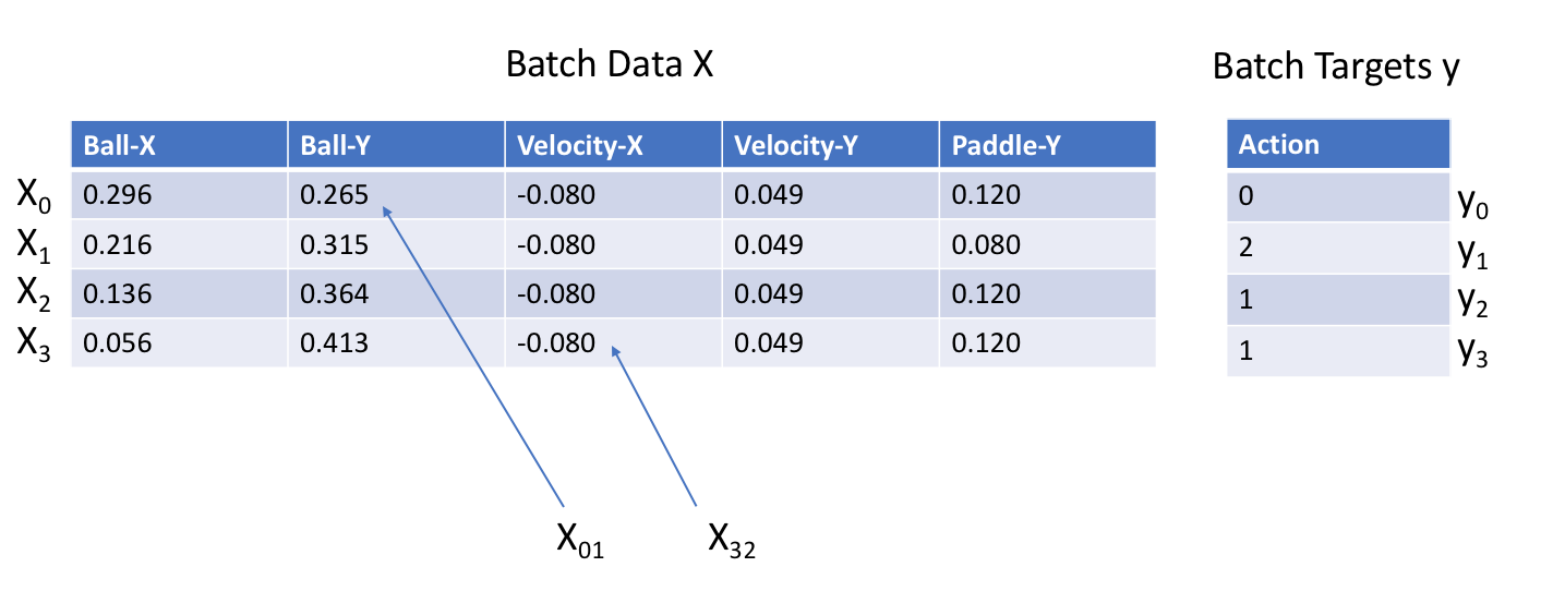
Note: You should find the batch size by yourself, but you do not need to justify the batch size you used.

Since we are using a gradient-based optimization algorithms, we want our loss to be differentiable. A common differentiable loss used for classification is softmax cross-entropy loss. More details about softmax cross entropy is given in this reference. We will give you the equations to implement the softmax cross-entropy loss in a later section.

Since we are using gradient descent, we want to compute the gradients of all weights and biases in the our model. Throughout the assignment we will be using the following notation. Let L be the loss function that we are trying to optimize over. Given an arbitrary 1d or 2d array V we will denote the derivative of V as "dV". If V is a 1d array, then dV_i is the derivative of L with respect to scalar V_i. If V is a 2d array, then dV_ij is the derivative of L with respect to scalar V_ij

Forward and Backward Propagation

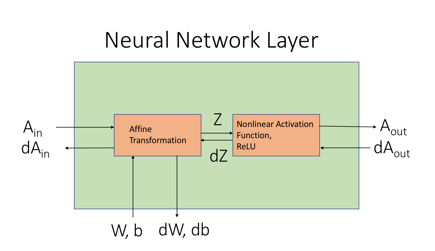
Neural networks run in two directions: forwards and backwards. Forward propagation uses the weights and biases at each layer to map the input to its estimate class. Backward propagation computes the gradients of the loss function with respect to the weights and biases at every layer using the chain rule. For every forward operation there is a backwards operation that computes the derivative of the forward operation using the chain rule from calculus. Here is a list of forward and backward functions that you will implement in this mp. You do not need to follow the function definitions explicitly, but make sure that you have the necessary functionality:

• Affine-Forward(A, W, b):
  • Description: Computes affine transformation Z = AW + b.
  • Inputs: Incoming batch of data A (2d array of size n x d), layer weight W (2d array of size d x d'), bias b (1d array of size d')
  • Returns: affine output Z (2d array of size nxd'), cache object
  • This function basically takes n training examples with d input features and creates a new dataset of n training examples with d' output features. A, W, and Z are 2d arrays and b is a 1d array. The number of output features d', also referred to as the number of layer units, is determined by you except for the last (output) layer, which must be 3. The function computes the following affine transformation.
    
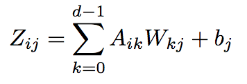
    Notice that this formula is just matrix multiplication between A and W with the addition of bias. The cache object is an object that stores the current values of A, W, and b. We need these values for the backwards operation.
• Affine-Backwards(dZ, cache):
  • Computes the gradients of loss L with respect to forward inputs A, W, b.
  • Inputs: Gradient dZ, cache object from forward operation
  • Returns: dA, dW, db
  • This function computes the gradients of A, W, and b with respect to loss. It is important to note that for any variable V and it's loss gradient dV have the same dimensions. Using the chain rule from calculus, the gradients dA, dW, and db are
    
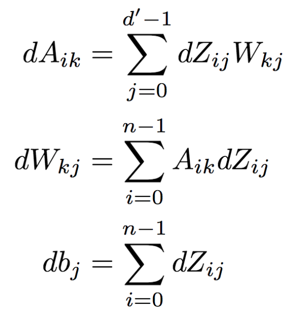
    The current values of A, W, and b are stored in the cache object from the forward operation.
• ReLU-Forward(Z):
  • Computes elementwise ReLU of Z.
  • Inputs: Batch Z (2d array of size n x d')
  • Returns: ReLU output A (2d array of size n x d'), cache object
  • The ReLU function takes the elements of some 2d array A and zeros out the values that are negative. Thus A_ij = Z_ij if Z_ij > 0, otherwise A_ij = 0. The cache object stores the value of Z since Z is needed for the ReLU backwards computation.
• ReLU-Backward(dA, cache):
  • Computes gradient of Z with respect to loss
  • Inputs: Gradient dZ, cache object from forward
  • Returns: gradient of Z with respect to loss L
  • If Z_ij was zeroed out during the ReLU forward computation, then the gradient dZ_ij must be 0 as well. This makes intuitive sense because if Z_ij was zeroed out, then Z_ij does not contribute to the loss L so the gradient of the loss L with respect to Z_ij must be 0. If Z_ij was not zeroed out, then dZ_ij = dA_ij.
• Cross-Entropy(F, y):
  • Description: Computes the loss function L and the gradients of the loss with respect to the scores F.
  • Inputs: logits and target classes
  • Returns: loss L and gradients dlogits.
  At every iteration the deep network outputs three scores per state one for each action. Let F_ik refers to the score of action k output by our neural network given the ith state in our batch X_i. Suppose y_i is the correct action that the agent should take at state X_i as labelled by the expert agent. The cross entropy-loss is given by the following equation where n is equal to the batch size and C is equal to the number of actions (in this case there are three actions). Note: F_iyi is the score output of our neural network for the ith example for "correct" action y_i.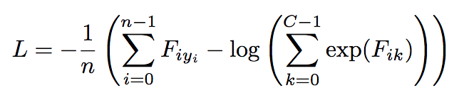
  Since we are using a gradient-based optimization procedure, we will also want to compute the gradients of the loss function with respect to the scores.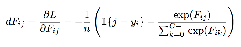

Here is example pseudocode that shows how to combine all the operations into a neural network. Note that W^p is the weight matrix (or 2d array) of the pth layer.

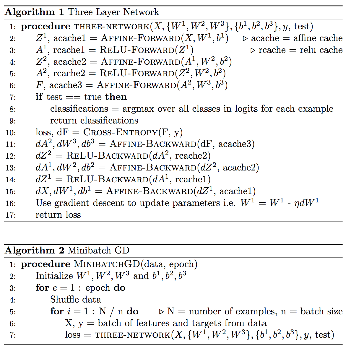
where, in line 16, you should use gradient descent to update all the parameters, not just W¹.

Weight and Bias Initialization and Normalization

Initializing the weights to be all 0's does not work; backpropagation will cause all weights to train to the same value. Can you see why? Instead, randomly initialize all your weight matrices between 0 and some weight scale parameter. This can be implemented by randomly initializing your weights between 0 and 1 and multplying by your weight scale parameter. You must find the correct weight scale parameter yourself. The bias term can be intialized to all 0's.

It may also helpful to center your dataset to 0 and scale the dataset to have a standard deviation of 1. Basically, you take every column of the dataset and subtract the mean of that column and divide by the standard deviation of that column. Although not strictly necessary it helped speed up our training process for part 2.1.

What You Need to Do For This Assignment

• Answer the following question in the report: What is the benefit of using a deep network policy instead of a Q-table (from part 1)? (Hint: think about memory usage and/or what happens when your agent sees a new state that the agent has never seen before).
• Implement the forward and backwards functions of a neural network and give a brief explanation of implementation and what neural network architecture you used.
• Train your neural network using minibatch gradient descent. Report the confusion matrix and misclassification error. You should be able to get an accuracy of at least 85% and probably 95% if you train long enough. Report you network settings including the number of layers, number of units per layer, and learning rate.
• Plot loss and accuracy as a function of the number of training epochs. You do not need to do a train-validation split on the data, but in practice this would be helpful.
• Run your pingpong agent with the trained policy. How many bounces does your agent achieve? You should get greater than 8 bounces averaged over 200 games although your results may be significantly higher. Your deep network agent does not need to beat your agent from part 1.

Tips

• Please shuffle your data after every training epoch.
• You are allowed and encouraged to use any linear algebra and numerical libraries, but you cannot use tensorflow or any autodifferentiation library for this part of the assignment. Autodifferentatiation is basically any feature that implements backpropagation for the user. Autodifferentiation is convenient, but understanding the concepts behind neural networks may be more useful in the long-run.
• Test modularly. Make sure your the function above work before trying to build and train your network. One way to check your backpropagation results is by implementing gradient checking. More details on gradient checking
• Recommended settings based on my implementation are a four layer neural network with 256 units per layer (except the last layer, which has 3) with a learning rate of 0.1. These settings are heavily implementation dependent. I use 300-500 epochs just to be safe so you should expect training to take about 2-10 minutes. You should also print results after every epoch to make sure things are running smoothly.

Part 2.2 Behavior Cloning Using Advantages Esimation (4pts for 4-unit students, 2pts extra credit for 3-unit students)

The deep neural network (DNN) you built in part 2.1 classifies states into action classes, but the neural network for this part will no longer be classifying states. Instead, the DNN should estimate the a quantity called "advantage" for every state and action using regression. The advantage of a state s and action a (A(s, a)) is the Q-value of s and a (Q(s, a)) subtracted by the value at state s (V(s)). Recall that the value of state s is the expected Q-value over all possible actions taken from a given state. That means that the A(s, a) tells you how much better action a is expected to be compared to average action you can take from state s.

The goal of regression is to estimate real, continuous outputs instead of discrete classes. Given a game state, your network should output three advantages for each of the three actions. When testing your agent, you should choose the action with the maximum advantage similiar to part 2.1. For part 2.2, the first five columns of the dataset are states, whereas the next three columns are the advantages for action 0, action 1, and action 2 respectively.
Data: expert advantage dataset

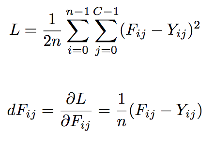
The significant difference between part 2.1 and part 2.2 is how we train the deep network. In part 2.1, we used a cross-entropy loss function, which is a loss function mostly used for classification. In part 2.2 since we are trying to predict real-valued outputs, we will use a mean-squared loss function, which measures the distance between each of our estimations and the expert advantages. The calculation of the loss function and the gradients of the loss are given below where F_{ij} is your advantage estimation and Y_{ij} is the target advantage for the ith state and jth action. Note that we use captial "Y" instead of lowercase "y" to indicate that "Y" is a 2d array and not a 1d array like in part 2.1.

For this part of the mp, you can get around the same number of bounces as you did in part 2.1. You should be able to achieve more than 8 bounces. Show the loss curve with respect to the number of epochs using minibatch gradient descent and describe the implementation and architecture of your dnn. Similar to part 2.1, I used the a four-layer architecture with 256 hidden units per layer. My learning rate was 0.1 and my weight scale intialization was 0.01. I also trained for 500 epochs.

Part 2: Extra Credit (2 points per section, up to a maximum 25 percent extra credit)

You are allowed to use an autodifferentiation framework for this extra credit portions of the assignment.

• Implement batch normalization for part 2.1. Including the forward and backwards operations. Report the number of bounces with and without batch normalization. If you are implemented
• Implement either dropout or any regularization scheme and split the data into 80%-20% train-validation split for part 2.1. Show the training and validation curves on the same plot with and without regularization, and report the best hyperparameters you achieved.
• Part 1 agent versus part 2. Let the agents from part 1 and part2 (2.1 or 2.2) compete. Report the results over 200 games. It does not matter which agent wins.

Report Checklist

Part 1.1: (for everybody)

1. Report and justify your choices for α, γ, exploration function, and any subordinate parameters. How many games does your agent need to simulate before it learns a good policy?
2. Use α, γ, and exploration parameters that you believe to be the best. After training has converged, run your algorithm on 200 test games and report the average number of times per game that the ball bounces off your paddle before the ball escapes past the paddle.
3. Include Mean Episode Rewards vs. Episodes plot for both Q-Learning and SARSA agents and compare these two agents.

Part 1.2: (for 4-unit students)

1. Describe the changes you made to your MDP (state space, actions, and reward model), if any, and include any negative side-effects you encountered after doing this.
2. Describe your method of training agent A and tell us why it works.
3. Include two Mean Episode Rewards vs. Episodes plots and compare these two agents.

Part 2.1: (for everybody)

1. Answer the following question in the report: What is the benefit of using a deep network policy instead of a Q-table (from part 1)? (Hint: think about memory usage and/or what happens when your agent sees a new state that the agent has never seen before).
2. Implement the forward and backwards functions of a neural network and give a brief explanation of implementation and architecture (number of layers and number of units per layer).
3. Train your neural network using minibatch gradient descent. Report the confusion matrix and misclassification error. You should be able to get an accuracy of at least 85% and probably 95% if you train long enough. Report you network settings including the number of layers, number of units per layer, and learning rate.
4. Plot loss and accuracy as a function of the number of training epochs. You do not need to do a train-validation split on the data, but in practice this would be helpful.
5. Report the number of bounces your agent gets. It should be around 8 bounces.

Part 2.2: (for 4-unit students, extra credit for 3-unit students)

1. Briefly describe the implementation of the Q-Network.
2. Report your choice for the best hyperparameters
3. Plot loss curve as a function of the number of episodes and report the number of bounces your agent gets averaged over 200 games. Full credit if greater than 8 bounces.

Submission Instructions

As usual, one designated person from the group will need to submit on Compass 2g by the deadline. Three-unit students must upload under Assignment 4 (three units) and four-unit students must upload under Assignment 4 (four units). Each submission must consist of the following two attachments:

1. A report in PDF format. As usual, the report should briefly describe your implemented solution and fully answer all the questions posed above. Remember: you will not get credit for any solutions you have obtained, but not included in the report.

   All group reports need to include a brief statement of individual contribution, i.e., which group member was responsible for which parts of the solution and submitted material.

   The name of the report file should be lastname_firstname_assignment4.pdf. Don't forget to include the names and NetIDs of all group members and the number of credit units at the top of the report.

2. Your source code compressed to a single ZIP file. The code should be well commented, and it should be easy to see the correspondence between what's in the code and what's in the report. You don't need to include executables or various supporting files (e.g., utility libraries) whose content is irrelevant to the assignment. If we find it necessary to run your code in order to evaluate your solution, we will get in touch with you.
   
   The name of the code archive should be lastname_firstname_assignment4.zip.

Multiple attempts will be allowed but in most circumstances, only the last submission will be graded. We reserve the right to take off points for not following directions.

Late policy: For every day that your assignment is late, your score gets multiplied by 0.75. The penalty gets saturated after four days, that is, you can still get up to about 32% of the original points by turning in the assignment at all. If you have a compelling reason for not being able to submit the assignment on time and would like to make a special arrangement, you must send me email at least four days before the due date (any genuine emergency situations will be handled on an individual basis).

Extra credit:

• We reserve the right to give bonus points for any advanced exploration or especially challenging or creative solutions that you implement. Three-unit students always get extra credit for submitting solutions to four-unit problems. If you submit any work for bonus points, be sure it is clearly indicated in your report.

Statement of individual contribution:

• All group reports need to include a brief summary of which group member was responsible for which parts of the solution and submitted material. We reserve the right to contact group members individually to verify this information.

WARNING: You will not get credit for any solutions that you have obtained, but not included in your report! For example, if your code prints out path cost and number of nodes expanded on each input, but you do not put down the actual numbers in your report, or if you include pictures/files of your output solutions in the zip file but not in your PDF. The only exception is animated paths (videos or animated gifs).

Be sure to also refer to course policies on academic integrity, etc.