
Detailed Instructions (Recommended Steps in Python)
-
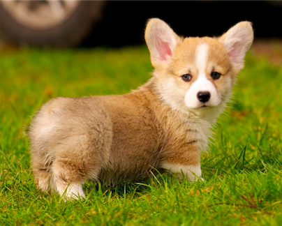
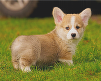
Here are two images. One has been lowpass filtered and
then downsampled by a factor of four in both the row and
column dimensions.
 Download them to your
computer (e.g., by right-clicking on the image and
choosing "save image to computer"). Read them in to
python using something like the following:
Download them to your
computer (e.g., by right-clicking on the image and
choosing "save image to computer"). Read them in to
python using something like the following:import scipy.ndimage as imgThe
corgibig=img.imread('corgibig.jpg')
corgismall=img.imread('corgismall.jpg')>
import matplotlib.pyplot as plt
plt.imshow(corgibig)
plt.title('Big Corgi')
plt.show()
plt.imshow(corgismall)
plt.title('Little Corgi')
plt.show()
plt.show()commands, here, force pyplot to generate a new set of axes for each new image, rather than trying to plot the images all on top of one another. -
Create a zero-insert upsampled image: an image with all of
the pixels from
corgismall, and with zero-valued pixels inserted in between. For example,
import numpy as npWhen I did this, I found that the image shown inside Spyder looks just like a bunch of dots, but that if I view the image in a real image reader, I can see that the corgi image has been spread out among all of the dots.
(nrs,ncs,ncolors)=corgismall.shape
corgiups=np.zeros((4*nrs,4*ncs,ncolors),dtype='uint8')
for m1 in range(0,nrs):
for m2 in range(0,ncs):
for color in range(0,ncolors):
corgiups[4*m1,4*m2,color]=corgismall[m1,m2,color]
plt.imshow(corgiups)
plt.title('Upsampled Corgi')
plt.show()
import scipy.misc
scipy.misc.imsave('corgiups.png',corgiups)
-
Create a piece-wise constant interpolation: instead of
filling all of the other pixels with zeros, fill them with
a copy of the nonzero pixel. For example,
	      corgipwc=np.zeros((4*nrs,4*ncs,ncolors),dtype='uint8')

	      for n1 in range(0,4*nrs):

	      for n2 in range(0,4*ncs):

	      for color in range(0,ncolors):

	      m1 = int(n1/4)

	      m2 = int(n2/4)

	      corgipwc[n1,n2,color]=corgismall[m1,m2,color]

	      plt.imshow(corgipwc)

	      plt.title('PWC Corgi')

	      plt.show()

	      scipy.misc.imsave('corgipwc.png',corgipwc)
-
Create a piece-wise linear interpolation: instead of
filling all of the other pixels with constants, fill them
with a linear interpolation of the four nearest nonzero
pixels (in images, this is sometimes called "bilinear
interpolation" because you do linear interpolation in two
directions). For example,
	      corgipwl=np.zeros((4*nrs,4*ncs,ncolors),dtype='uint8')

	      for n1 in range(0,4*nrs):

	      m1 = int(n1/4)

	      g1 = 1-0.25*(n1-4*m1)

	      m1p1 = min(nrs,m1+1)

	      for n2 in range(0,4*ncs):

	      m2 = int(n2/4)

	      g2 = 1-0.25*(n2-4*m2)

	      m2p1 = min(ncs,m2+1)

	      for color in range(0,ncolors):

	      corgipwl[n1,n2,color]=g1*g2*corgismall[m1,m2,color]

	      corgipwl[n1,n2,color]+=g1*(1-g2)*corgismall[m1,m2p1,color]

	      corgipwl[n1,n2,color]+=(1-g1)*g2*corgismall[m1p1,m2,color]

	      corgipwl[n1,n2,color]+=(1-g1)*(1-g2)*corgismall[m1p1,m2p1,color]

	      plt.imshow(corgipwl)

	      plt.savefig('corgipwl.png')
-
Use the scipy FFT function to create a log-magnitude
spectrum of the first row of each image, including the
input high-resolution image, the input low-resolution
image, and all three of the images you have created. Plot
them all on the same axes, using different color lines.
Note that you'll have to use a different frequency axis
for the input low-resolution image than for all the
others. Before you apply
math.log10, you'll need to make sure the FFT absolute value is nonzero; it turns out that clipping at 1 is a reasonable thing to do for these spectra, since few of them are below 1 in magnitude. Also, I recommend that you add 1 to each successive spectrum, so that they don't sit right on top of one another, so that you can see them. For example, notice the +1, +2, +3 and +4 in this code:
import scipy.fftpack as fftNotice that the small spectrum takes the first pi/4 radians of the big spectrum, and stretches them out to pi. The upsampled image takes the entire small image, and repeats it exactly, four times. The PWC and PWL spectra are like the upsampled spectrum, but with the aliasing damped out a lot.
import math
specbig = [ 20*math.log10(max(1,abs(x))) for x in fft.fft(corgibig[0,:,0]) ]
specups = [ 20*math.log10(max(1,abs(x)))+1 for x in fft.fft(corgiups[0,:,0]) ]
specpwc = [ 20*math.log10(max(1,abs(x)))+2 for x in fft.fft(corgipwc[0,:,0]) ]
specpwl = [ 20*math.log10(max(1,abs(x)))+3 for x in fft.fft(corgipwl[0,:,0]) ]
specsmall = [ 20*math.log10(max(1,abs(x)))+4 for x in fft.fft(corgismall[0,:,0]) ]
omegabig = [ 2*math.pi*k/(4*ncs) for k in range(0,4*ncs) ]
omegasmall = [ 2*math.pi*k/ncs for k in range(0,ncs) ]
plt.plot(omegasmall,specsmall,'r',omegabig,specbig,'g',omegabig,specups,'b',omegabig,specpwc,'k',omegabig,specpwl,'m')
plt.xlim((0,2*math.pi))
plt.ylim((20,80))
plt.xlabel('Frequency (radians/sample)')
plt.title('G=big, R=small, B=upsampled, K=PWC, M=PWL')
plt.savefig('corgispectra.png')
Deliverables (Required)
By 2/14/2017 23:59, upload to compass a zip file named MYNAME_LAB4.ZIP containing the following things:
- Three images: zero-insert upsampled, PWC, and PWL interpolated.
- An image file showing the log average row spectra of your three created images, of the original image, and of the small image, in different colored lines on the same axes.
- A program that reads in the two input images, and creates the four upsampled images and the spectral plot.
Walkthrough
The video walkthrough is here.