The goal of this project is to familiarize yourself high dynamic range (HDR) imaging, image based lighting (IBL), and their applications. By the end of this project, you will be able to create HDR images from sequences of low dynamic range (LDR) images and also learn how to composite 3D models seamlessly into photographs using image-based lighting techniques. HDR tonemapping can also be investigated as bells and whistles.
HDR photography is the method of capturing photographs containing a greater dynamic range than what normal photographs contain (i.e. they store pixel values outside of the standard LDR range of 0-255 and contain higher precision). Most methods for creating HDR images involve the process of merging multiple LDR images at varying exposures, which is what you will do in this project.
HDR images are widely used by graphics and visual effects artists for a variety of applications, such as contrast enhancement, hyper-realistic art, post-process intensity adjustments, and image-based lighting. We will focus on their use in image-based lighting, specifically relighting virtual objects. One way to relight an object is to capture an 360 degree panoramic (omnidirectional) HDR photograph of a scene, which provides lighting information from all angles incident to the camera (hence the term image-based lighting). Capturing such an image is difficult with standard cameras, because it requires both panoramic image stitching (which you will see in project 5) and LDR to HDR conversion. An easier alternative is to capture an HDR photograph of a spherical mirror, which provides the same omni-directional lighting information (up to some physical limitations dependent on sphere size and camera resolution). We will take the spherical mirror approach, inspired primarily by Debevec's paper. With this panoramic HDR image, we can then relight 3D models and composite them seamlessly into photographs. This is a very quick method for inserting computer graphics models seamlessly into photographs and videos; much faster and more accurate than manually "photoshopping" objects into the photo.
Terminology
First, let's review some of the key terms and concepts:
Irradiance is the amount of light received per second by the sensor cell. If you take multiple pictures with different exposure times, the irradiance should still be constant for a given pixel, assuming the scene lighting hasn't changed between pictures.
Exposure Time or "shutter time" is the amount of time that the shutter is open, typically a fraction of a second.
Exposure is the amount of light that reaches the sensor while the shutter is open, which is the product of irradiance and exposure time.
Intensity here refers to the pixel value that is recorded in the original images. The intensity is a non-linear function of exposure (according to the camera response function) and can be clipped if the exposure is very large or small.
Recovering HDR Radiance Maps (70 pts)
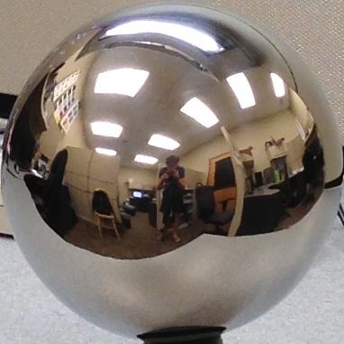
To the right are three pictures taken with different exposure times (1/24s, 1/60s, 1/120s) of a spherical mirror in an office. The rightmost image shows the HDR result (tonemapped for display). In this part of the project, you'll be creating your own HDR images. First, you need to collect the data.
What you need:
Spherical mirror
Camera with exposure time control. This is available on all DSLRs and most point-and-shoots, and even possible with most mobile devices using the right app; e.g. ProCamera on iOS, Camera FV-5 Lite on Android (this even has auto exposure bracketing, AEB). Automatic exposure bracketing is helpful but not really needed.
Tripod or rigid surface to hold camera or very steady hand (not recommended)
Data collection (20 points)
You can use our provided samples for this project (see samples folder and readme in materials), or collect your own which is much more interesting and will earn you 20 points. If you use the provided LDR samples to compute the HDR map, you must still use your own background image for the synthetic object rendering later.
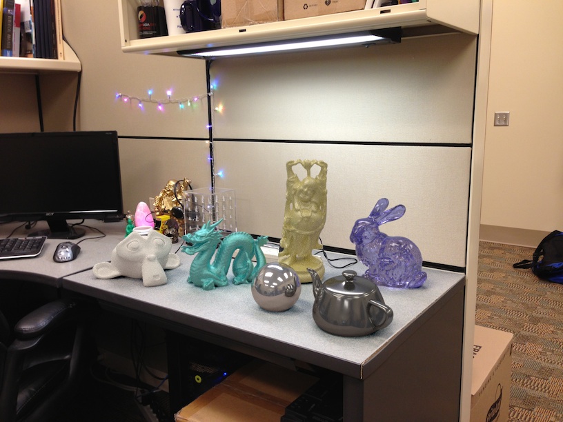
Find a good scene to photograph. The scene should have a flat surface to place your spherical mirror on (see my example below). Either indoors or outdoors will work.
Find a fixed, rigid spot to place your camera. A tripod is best, but you can get away with less. I used the back of a chair to steady my phone when taking my images.
Place your spherical mirror on a flat surface, and make sure it doesn't roll by placing a cloth/bottle cap/etc under it. Make sure the sphere is not too far away from the camera -- it should occupy at least a 256x256 block of pixels.
Photograph the spherical mirror using at least three different exposure times. Make sure the camera does not move too much (slight variations are OK, but the viewpoint should generally be fixed). For best results, your exposure times should be at least 4 times longer and 4 times shorter (±2 stops) than your mid-level exposure (e.g. if your mid-level exposure time is 1/40s, then you should have at least exposure timess of 1/10s and 1/160s; the greater the range the better). Make sure to record the exposure times.
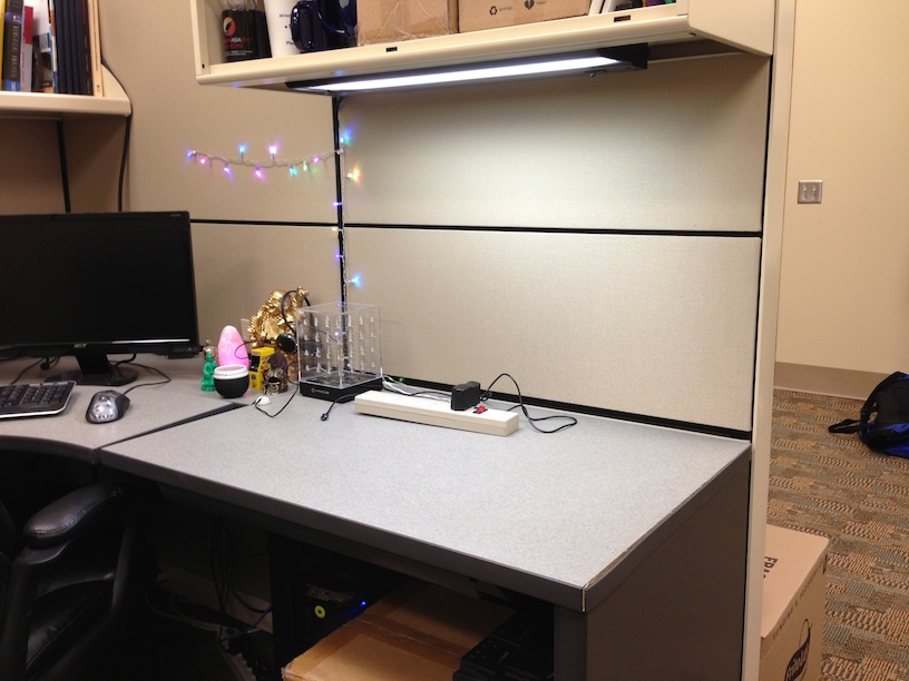
Remove the mirror from the scene, and from the same viewpoint as the other photographs, take another picture of the scene at a normal exposure level (most pixels are neither over- or under-exposed). This will be the image that you will use for object insertion/compositing (the "background" image).
After you copy all of the images from your camera/phone to your computer, load the spherical mirror images (from step 4) into your favorite image editor and crop them down to contain only the sphere (see example below).
Small alignment errors may occur (due to camera motion or cropping). One way to fix these is through various alignment procedures, but for this project, we won't worry about these errors. If there are substantial differences in camera position/rotation among the set of images, re-take the photographs.
From left to right: one of the sphere pictures (step 4), cropped sphere (step 6), empty scene (step 5)
Naive LDR merging (10 points)
After collecting data, load the cropped images, and resize them to all be square and the same dimensions (e.g. cv2.resize(ldr,(N,N)) where N is the new size). Either find the exposure times using the EXIF data (usually accessible in the image properties), or refer to your recorded exposure times. To estimate the irradiance for each image (up to a scale), divide each intensity by its exposure time (e.g. ldr1_irradiance = ldr1 / exposure_time1). This assumes a direct linear relationship between intensity and total exposure, which is not quite right, but will do for now. Different LDR images will produce different irradiance estimates, so for the naive method, simple compute the average irradiance for each pixel and channel to get your "naive" estimate.
To save the HDR image, use the provided write_hdr_image function. To visualize HDR image, you will need to write a display_hdr_image function that maps an arbitrary range to 0 to 1. Some recommendations are made in the Jupyter notebook.
Weighted LDR merging (15 points)
The naive method has an obvious limitation: if any pixels are under- or over-exposed, the result will contain clipped (and thus incorrect) information. Instead of using an unweighted average, create a weighting function (or array) that maps each pixel intensity into a weight, where pixel values close to 0 or 255 (in a 0 to 255 range) have weights close to 0, and pixel intensities close to 128 have weights close to 1. One such weighting function is w = lambda z: float(128-abs(z-128)) assuming pixel values range in [0,255]. Note that the weight is a function of intensity, but the sum is over irradiance, which can have larger values than maximum LDR intensity. To compute a weighted average of irradiance, compute a weighted sum of irradiances and then divide by the sum of weights for each pixel.
LDR merging with camera response function estimation (15 points)
In practice, intensity is a non-linear function of exposure both due to clipping and due to the camera response function, which for most cameras compresses very dark and very bright exposure readings into a smaller range of intensity values. To convert pixel values to true radiance values, we need to estimate this response function. Since we have multiple observations of each pixel with different exposure times, we can solve for the irradiance (exposure per second) at each pixel up to an unknown constant factor.
The method we will use to estimate the response function is outlined in this paper. Given pixel intensity values Z at varying exposure times t, the goal is to use the constraint g(Z) = ln(R*t) = ln(R)+ln(t) to solve for log R (log irradiance) for each pixel and g(Z), the mapping from an intensity to log exposure. By these definitions, g is the inverse log response function. The paper provides code to solve for g given a set of pixels at varying exposures (we also provide gsolve function in our utils folder). Use this code to estimate g for each RGB channel. Then, recover the HDR image using equation 6 in the paper.
Some suggestions on using gsolve:
When providing input to gsolve, don't use all available pixels, otherwise you will likely run out of memory / have very slow run times. To overcome, just randomly sample a set of pixels (1000 or so can suffice), but make sure all pixel locations are the same for each exposure.
The weighting function w should be implemented using Eq. 4 from the paper (this is the same function that can be used for the previous LDR merging method).
Try different lambda values for recovering g. Try lambda=1 initially, then solve for g and plot it. It should be smooth and continuously increasing. If lambda is too small, g will be bumpy.
Refer to Eq. 6 in the paper for using g and combining all of your exposures into a final image. This produces log irradiance values, so make sure to exponentiate the result and save irradiance in linear scale.
Additional questions to answer in your report (10 points)
The starter notebook includes code to compare the consistency of the irradiance estimates from each image and the dynamic range of the final HDR result. In my own results, each subsequent version of HDR estimation provides more consistent irradiance estimates per image and a greater dynamic range. In your report, answer these questions:
For a very bright scene point, will the naive method tend to over-estimate the true brightness, or under-estimate? Why?
Why does the weighting method result in a higher dynamic range than the naive method?
Why does the calibration method result in a higher dynamic range than the weighting method?
Why does the calibration method result in higher consistency, compared to the weighting method?
Panoramic transformations (10 points)
Now that we have an HDR image of the spherical mirror, we'd like to use it for relighting (i.e. image-based lighting). However, many programs don't accept the "mirror ball" format, so we need to convert it to a different 360 degree, panoramic format (there is a nice overview of many of these formats here). Most rendering software accepts this format, including Blender's Cycles renderer, which is what we'll use in the next part of the project.
To perform the transformation, we need to figure out the mapping between the mirrored sphere domain and the equirectangular domain. We can calculate the normals of the sphere (N) and assume the viewing direction (V) is constant. We then calculate reflection vectors with R = V - 2 * dot(V,N) * N, which is the direction that light is incoming from the world to the camera after bouncing off the sphere. The reflection vectors can then be converted to spherical coordinates by providing the latitude and longitude (phi and theta) of the given pixel (fixing the distance to the origin, r, to be 1). This assumes an orthographic camera (which is a close approximation as long as the sphere isn't too close to the camera). The view vector is assumed to be at (0,0,-1).
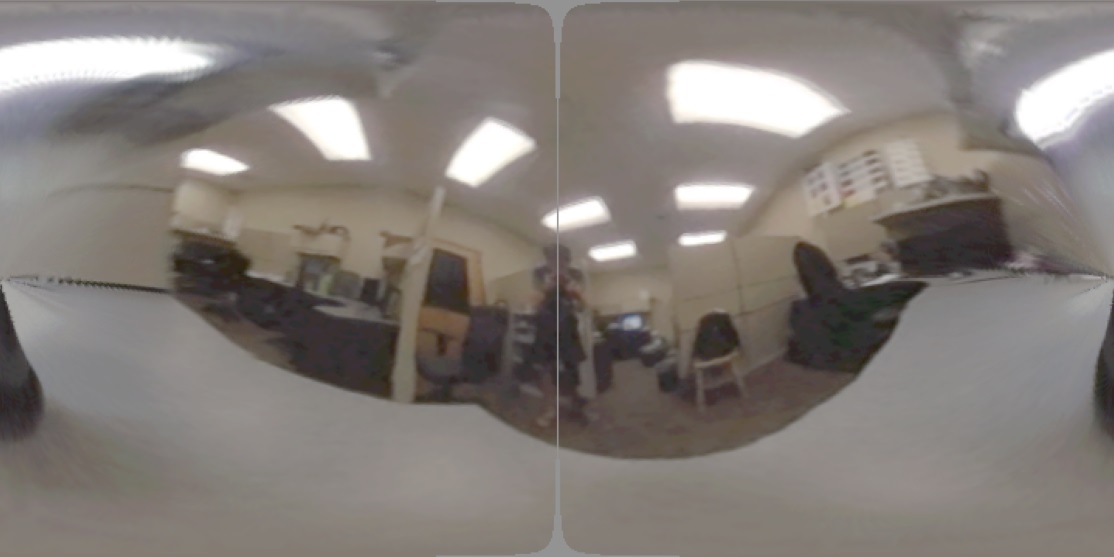
Next, the equirectangular domain can be created by making an image in which the rows correspond to theta and columns correspond to phi in spherical coordinates. For this we have a function in the starter code called get_equirectangular_image (see the function under utils in hdr_helpers.py). The function takes reflection vectors and the HDR image as input and returns the equirectangular image as output. Below is an example result.
Rendering synthetic objects into photographs (30 pts)
The steps to render the synthetic objects using Blender 2.8 are described on this page and this demo video. Be sure to use your own background image for this, even if you created the HDR map out of the samples.
Another 10 points are allocated for quality of results.
Bells & Whistles (Extra Points)
Additional Image-Based Lighting Result (20 pts)
For 10 points, create an image-based lighting result with an interesting set of objects using the same HDR light map as your main result. These objects should not all be default Blender objects and can be from online sources. For 10 points, create a result with the same objects but a different lighting map to see its effects. These two additional result images can be worth 20 points total.
Other panoramic transformations (20 pts)
Different software accept different spherical HDR projections. In the main project, we've converted from the mirror ball format to the equirectangular format. There are also two other common formats: angular and vertical cross (examples here and here). Implement these transformations for 10 extra points each (20 possible).
Photographer/tripod removal (25 pts)
If you look closely at your mirror ball images, you'll notice that the photographer (you) and/or your tripod is visible, and probably occupies up a decent sized portion of the mirror's reflection. For 25 extra points, implement one of the following methods to remove the photographer: (a) cut out the photographer and use in-painting/hole-filling to fill in the hole with background pixels (similar to the bells and whistles from Project 2), or (b) use Debevec's method for removing the photographer (outlined here, steps 3-5; feel free to use Debevec's HDRShop, if available, for doing the panoramic rotations/blending). The second option works better, but requires you to create an HDR mirror ball image from two different viewpoints, and then merge them together using blending and panoramic rotations.
Local tonemapping operator (25 pts)
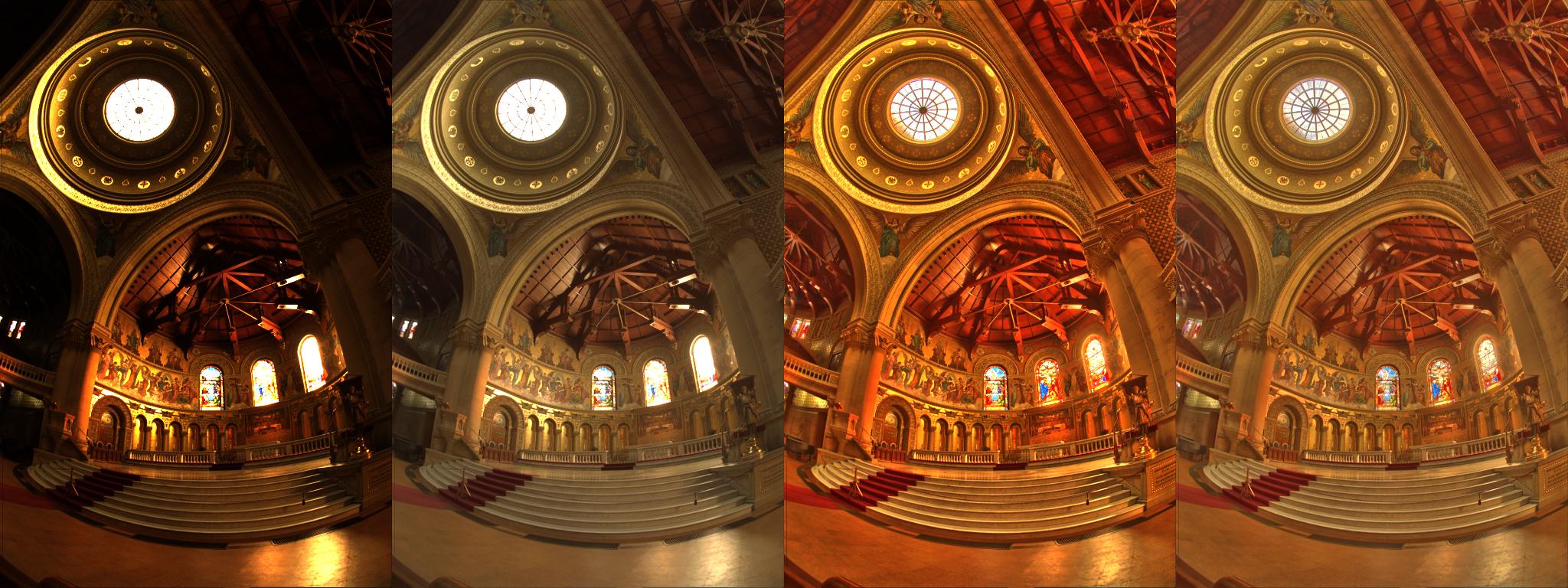
HDR images can also be used to create hyper-realistic and contrast enhanced LDR images. This paper describes a simple technique for increasing the contrast of images by using a local tonemapping operator, which effectively compresses the photo's dynamic range into a displayable format while still preserving detail and contrast. For 25 extra credit points, implement the method found in the paper and compare your results to other tonemapping operations (see example below for ideas). We provide you bilateral_filter function, but do not use any other third party code. You can find some example HDR images here, including the memorial church image used below.
From left to right: simple rescaling, rescaling+gamma correction, local tonemapping operator, local tonemapping+gamma correction.
To turn in your assignment, download/print your Jupyter Notebook and your report to PDF, and ZIP your project directory including any supporting media used. See project instructions for details. The Report Template (above) contains rubric and details of what you should include.
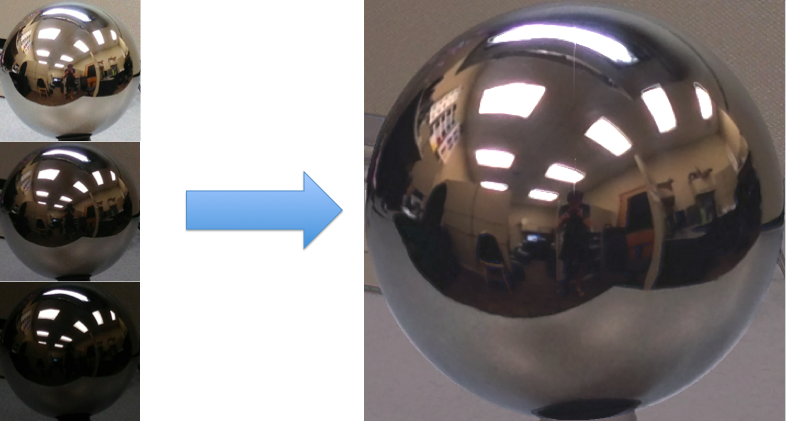 To the right are three pictures taken with different exposure times (1/24s, 1/60s, 1/120s) of a spherical mirror in an office. The rightmost image shows the HDR result (tonemapped for display). In this part of the project, you'll be creating your own HDR images. First, you need to collect the data.