CS357 Numerical Methods I
Summer 2014
Machine Problem 1
Posted: June 18th, 2014
Due Date: 9:00 P.M., Friday June 27th, 2014
The score for MP 1 will be based on the results from the mp1_check program. No hand grading will be performed on any MP work submitted!
Handin now available here.
Part 1: Designing a Suspension Bridge
1. Introduction
This Machine Problem involves designing a suspension bridge using slinky springs. Given the number of springs (N+1), the total length of all the springs (L), the weights the vertical supporting cables will maintain (W, a vector), and the horizontal distances between the vertical supporting cables (d, a vector), attached in the manner presented in the figure below, your goal is to compute the length of each of the vertical supporting cables (h, a vector). Springs are connected in series (the points that they connect together are called joint points). The two ends of the slinky chain are attached to the left and the right towers. The formulas modeling this problem are given below. Briefly decribed, your program requestes an initial guess from the user for HF , the horizontal force in the slinky chain. Given horizontal force HF, the spring constants (K, a vector) can be computed from the horizontal distances (d, a vector). Once the spring constants K have been determined, the system of equations for the vertical positions h can be computed. Finally, the lengths of all the individual springs can be computed and the maximum length found.
Of course, if the user guessed an incorrect value of HF then our results are incorrect. We can check for a correct HF by calculating the sum of the lengths of all the springs and this should be equal to L. Rather than repeating a guess for HF we will use the SciPy library function named scipy.optimize.fsolve to compute the true HF.
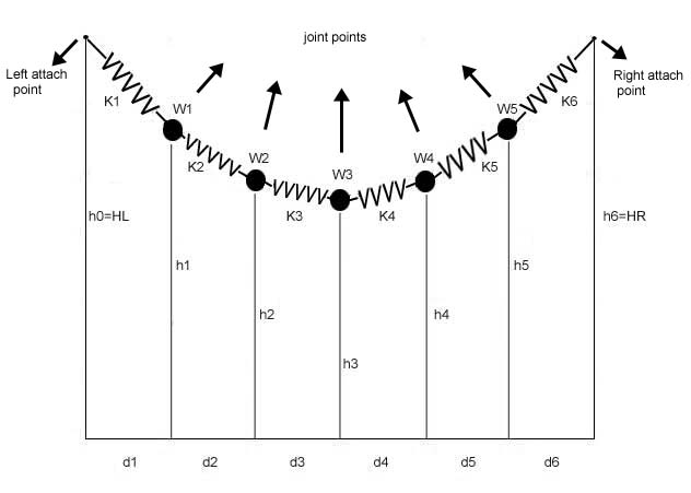
Figure 1. A model of the suspension bridge
Figure 1 shows a system with five weights. Nevertheless, your program should handle any numbers of weights, not just five. The forces from the deck of the bridge are depicted as point masses labeled Wi.
2. Preparation
a) Before you start working on the MP make sure you have a good understanding of Python and NumPy and SciPy (Python names ) and Matplotlib (more Resources).
b) Download the following files and save them to your home directory:
-
A complete working demo program mp1_demo . The demo program demonstrates how your program should run. After you finish coding, you can run your own program and compare its output with the output of the demo program.
-
The data characterizing the bridge are provided in the file mp1_data.py ( a script not a function).
The file mp1_data.m contains the following variables:
-
N: The number of weights used in the system
-
d: A row vector containing the distances between each weight (Length: N+1)
-
W: A column vector containing the weights used in the system (Length: N)
-
HL: The height of the left attach point (left tower)
-
HR: The height of the right attach point (right tower)
-
L: The (target) sum of the lengths of all the springs.
After opening Python, run the mp1_data.py script by typing
from mp1_data import *
at the Python prompt. After running the script, check to make sure that the variables N, d, W, HL, HR and L have been defined for you to use in Pyhton. Feel free to modify the values in mp1_data to test if your program can handle varying values.
c) To see how your program should work, at the Linux prompt type (don't type the $):
$ module load python3
$ python3 mp1_demo.cpython-34.pyc
where the $ symbol corresponds to your Linux comand line prompt (which may differ from user to user).
You can also add a line 'module load python3' to your '~/.bashrc' file so you don't have to enter 'module load python3' each time you open a new terminal.
3. Math
This section explains the math you need to construct the suspension bridge. Some of the equations derived in this section will be referenced later when you write your code.
We need to calculate the heights of the support cables: [h1 h2 h3 ... hN]
First, focus on only one weight Wi in the system:
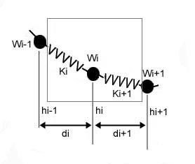
Figure 2. Model of one weight in the system
If you resolve the forces acting on the system (above) at Wi you have a figure that looks like the following:
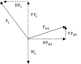
Figure 3. Forces acting on the system
The force from the vertical cable exerts a force Wi in the downward direction . Since the system is in a stable state, we resolve the forces acting on Wi into vertical and horizontal components:
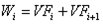 (1)
(1)
Since all the forces acting in the horizontal direction are equal, we can call all of them HF.
 (2)
(2)
Considering the forces in the horizontal direction, from Hooke's law, we can conclude:
 (3)
(3)
(Horizontal force only concerns the displacement in x-direction. )
If we guess HF and d (vector) is given ( in mp1_data.m), then we can compute K (vector) as:
 (4)
(4)
Considering the forces acting in the vertical direction, from Hooke's law, we can write,
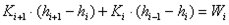 (5)
(5)
Given Wi and Ki for i = 1,2,3,...,N, we then have N linear equations of N unknowns (h1 to hN), which forms a linear system. These equations define a tri-diagonal system of linear equations for the heights h1 to hN of the weights W1 to WN. Note that h0 is the given HL while hN+1 is HR. Solving this system of equations, we arrive at the general equation for the system (in matrix form):
 (6)
(6)
where lhs is an N-by-N matrix, while both h and rhs are N-by-1 vectors as follows :

We solve the system by solving the matrix equation,
 (7)
(7)
You will also need to solve for the magnitude of Fi for each individual spring in the system. Then pick the maximum magnitude as a solution. In order to compute the maximum magnitude of Fi you will use the formula,
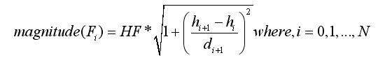 (8)
(8)
4. Implementation
You have to create six files (modules): main.py, xy_length.py, find_xy.py, diff_L.py, final_graphs.py and max_force.py.
The table below summarizes what are the functions that you need to write, what files do you have to store them in, and what are the operations for each function.
|
Name of function
|
Store in file
|
Function operation |
|
xy_length |
xy_length.py
|
Computes the total length of the spring chain. (step 1)
|
|
find_xy
|
find_xy.py
|
Computes the x and y coordintates for both the joint and attach points. (step 0)
|
|
diff_L |
diff_L.py
|
Computes the differnce between the target and calculated length of the spring chain. (step 2)
|
|
max_force
|
max_force.py
|
computes the magnitude of the force Fi of each spring and returns the maximum one. (step 5)
|
|
main |
main.py |
to execute MP1 call main with a single input argument HF. The output of main is x and y. (step 3) |
|
final_graphs |
final_graphs.py |
Plots values from Data (global variable) showing how fzero obtains solution true_HF given guess HF. (step 4) |
This section describes how to implement above functions in a step-by-step fashion. (Note: your program should be able to handle any number of weights. Please make your functions generic.)
Step 0 Download skeleton files
Download the file skeleton.py.tar.gz and open this tar file by typing the following command at the Linux terminal window.
tar -xzvf skeleton.py.tar.gz
Step 1 find_xy
Using an editor (either gedit, vim or idel ) open the file find_xy.py. The find_xy function has one input HF.
Using HF and d create a list K according to equation (4).
Use
np.diag() to create three matrices, upper, lower and main such that lhs = upper+lower+main (the matrix shown in the diagram below (6))
Copy (using
W.copy() ) the values of W into rhs.
Modify the first and last elements of rhs according to the figure below (6).
Use
np.linalg.solve() to solve the system of linear equations as in (7).
Create a vector x of x-coordinates based on the vector of values d found in mp1_data. Take the x coordinate of the leftmost point to be 0. Use
np.append() and
np.cumsum() to do this.
Create a vector y of y-coordinate values based on the vector of values h we just calculated and HL and HR found in mp1_data. Use
np.append() to append the values HL and HR at beginning and end.
Unit test: At the Linux prompt type:
$ module load python3
$ python3 find_xy.py
Then you should get the following values for x and y:
X = [ 0. 7.5 15. 22.5 30. 37.5 45. 52.5 60. 67.5 75. ]
(grader: 5 points all or nothing)
Y = [ 70. 56.65 45.8 37.45 31.6 28.25 27.4 29.05 33.2 39.85 50. ]
(grader: 5 points all or nothing)
Step 2 xy_length
The purpose of the function xy_length is to calculate the sum of the distances between the points contained in the two vectors that are given to it as input. The function has two input parameters x and y, which are vectors, and its return value is a single variable (let's call it total), that represents the sum of the Euclidean distances between each consecutive pair of points. Use
np.diff() and
np.sqrt() to perform this calculation.
Unit Test: At the Linux prompt type:
$ module load python3
$ python3 xy_length.py
This calculates the distance between the points (0,0), (3,4) and (6,8).
You should get the answer as:
Length = 10.0
(grader: 6 points all or nothing)
Step 3 diff_L
This function has one input, HF. The purpose of this function is to compute the difference, between the target length L and the total length of the springs running from the left tower to the right tower. The input argument to this function is the guesstimate of the horizontal force, HF, and the return value is L - calclength, the error in your approximation of the length of springs needed for you bridge. Your function should perform the followin
-
Import the values defined in mp1_data.py. This is already done for you using the from-import command.
-
Data is a global variable declared in mp1_data.py which must be modified by this function. Use the global command. This is already done for you.
-
Call the function find_xy using the horizontal force HF. A call of find_xy returns two vectors of coordinates of the topmost points of the vertical cables (including the towers). Store them in two vectors; x and y.
-
Use these vectors, x and y as input arguments and call xy_length, to find the sum of the lengths of the springs between the left tower and the right tower. Store the return value of xy_length in a variable; calc_length.
-
Plot or update a figure to show the x,y coordinates for this iteration. This gives a visualization of the progression of the xy coordinates from the initial system based on the estimated HF values as Diff_L is called repeatedly.
if handle == None:
fig = pt.figure(1)
# use pt.xlabel(), pt.ylabel() and pt.title() to assign values as in the demo.
# Plot x and y. Your plot command should look like this:
handle, = pt.plot(x,y,'b-o', mec='k', mfc='g', ms=10)
pt.show(block=False)
else:
handle.set_data(x,y)
pt.draw()
-
Pause the program 0.1 seconds. Use time.sleep(0.1). This pause allows the updates to xy to be slower, creating an animation effect.
-
Update the global variable Data that you're using to store the horizontal force and the calculated length for each of the iterations. Basically, we want to append two values (HF , calc_length) as the next row of Data during each iteration (i.e. during each call to this function). Each of the two values should be added as a new row to Data. Take the Data that existed from the previous iterations, and append the HF and calc_length from this iteration to it. This will create a timeline of horizontal forces and lengths. We'll use this later to plot how we approached the optimal answer.
The variable Data should therefore be a matrix with i rows and 2 columns; where i is the number of iterations we perform. The first element in each row (the entire first column) will contain the horizontal forces that you calculate at each iteration, and the second element in each row (the entire second column) will contain the springs lengths that you calculate at each iteration.
After i iterations, Data should have this structure:
    Data = [ [ HF1,  calc_length1 ]
             [ HF2,  calc_length2 ]
             [ HF3,  calc_length3 ]
                ... ...
             [ HFi,  calc_lengthi ] ]
Use append() on Data to append the values HF and calc_length.
-
return L - calc_length # we have included this code for you.
Unit Test: At the Linux prompt type:
$ module load python3
$ python3 diff_L.py
Call diff_L with the initial value of 20.
You should get the answer as:
b = 6.3739801917
and there should be a correct label on the horizontal and vertical axis along with a correct title. (grader: 13 points total, 7 for correct b, 2 points for each label and title)
Step 4 final_graphs
Since we're applying an iterative process to get to the optimal solution, we'd be interested in knowing how we approached that solution. That's what this function is going to do. It does not accept any input parameters and does not return any values. The function definition line should look like this:
def final_graphs():
-
Import the data from mp1_data.py. We have coded this step for you.
-
final_graphs is definitely going to want to access the information in our global vector Data, so make Data visible by declaring it as global here too.
-
Open a new figure window:
pt.figure(2)
-
Split the matrix Data into two vectors Forces and Lengths as follows:
Create a vector Forces that has all the forces that were in Data. To do this, you need to access the first column in every row of Data (i.e. the first column).
Create a vector Lengths that has all the lengths that were in Data. To do this, you need to access the second column in every row of Data (i.e. the second column).
Yes, there is a simple way to do this!
-
Use pt.plot() to plot a graph of Lengths vs. Forces (FYI: When we say 'plot y vs. x', we mean plot(x,y) ). Use 'r*', ms=10, label='Forces'.
-
Plot a horizontal line using pt.axhline(y=L, ls='-', color='b', label='Lengths').
-
Display the legend; use pt.legend(loc='best').
-
Set the title of the graph to be 'Lengths vs. Forces'. Label the X axis as 'Forces'. Label the Y axis as 'Lengths'. Use the pt.xlabel(), pt.ylabel(), pt.title() functions.
-
Open a third figure window.
-
Create an array of values from 1 to the number of rows in the Data matrix. To do this complete the code for
iterations = np.arange(1, _________your code here___________)
Note tha if A is an array then A.size returns one less than the number of elements in A.
-
Plot Lengths versus iterations. Use 'r*', ms=10, label='Lengths'.
-
Plot Forces versus iterations. Use 'g*', ms=10, label='Forces'.
-
As in step 6, use pt.axhline() to plot a horizontal line. Use label='True length'.
-
Set the title of the graph to be 'Lengths vs. Iterations'. Label the X axis as 'Iterations'. Label the Y axis as 'Lengths'.
-
Display the legend.
-
Display the graphs using pt.show()
Unit Test:
The test for final_graphs is included in the test for main (see below).
Step 5 max_force
The max_force function will determine the maximum magnitude of the Fi for any of the springs. This function should have two input parameters: h and HF . See the equation (8) in the Math section 3 above.
1. The function definition line for max_force is:
def max_force(h,HF):
2. Use the functions
max(),
np.diff() and
np.sqrt() to find the maximum force and assign the result to the output variable named F .
Unit Test:
The test for max_F is included in the test for main (see below).
Step 6 main
This is the function that you will actually call when you run the program as a whole. The function accepts one input parameter, HF, and it returns two vectors x and y, and two values, true_HF and max_F. The function definition line should look like this:
def main(HF):
That is, when you type in the following at the command prompt, the program should run and give you the output you expect, plus the graphs.
$ module load python3
$ python3
>>> from main import main
>>> main(12)
-
Use optimize.fsolve() to find a root (or a zero) of diff_L using an initial value of HF, and store the value returned in a variable true_HF. Note that we imported optimize from scipy.
-
Call the function find_xy with true_HF as it's argument, and store the values returned in vectors x and y.
-
Call the function final_graphs to plot your progression from the initial guess to the optimal solution. If you want to test everything you've written till this point, before going on to write final_graphs, you can do so, you just won't be able to see all of the figures that you'll need in the end. Just leave this line out for the time being, and insert it when you have written final_graphs.py.
-
Call the max_force function (you will write in step 5).
max_F = max_force(y, true_HF);
-
return x, y , true_HF, max_F # this has been coded for you
Unit Test:
At the Linux prompt type:
$ module load python3
$ python3 main.py
Call main with the initial value of 10.0 as above.
You should get the answer as:
X = [ 0. 7.5 15. 22.5 30. 37.5 45. 52.5 60. 67.5 75. ]
Y = [ 70. 57.67802563 47.62961389 39.8547648 34.35347833 31.12575451 30.17159332 31.49099477 35.08395886 40.95048558 50. ]
true_HF = [ 16.49393748]
max_F = 31.7233723424
and there should be three correct plots. (grader: 21 points total, 2 points for X, 2 points for Y, 4 points for true_HF and 4 points for max_F and 9 points for the plots (that is 3points for each of three plots).
5. Grading Scheme
Everything working perfectly (correct answers and graphs plotted right) = 50 points. The grading is based on a per function basis. The table below lists points per function.
|
Function |
Points |
|
find_xy |
10 |
|
max_force |
|
|
xy_length |
6 |
|
diff_L |
13 |
|
main |
21 |
|
final_graphs |
|
Hand in Procedure
That's it! You're done!!!