Errors and Complexity
Learning objectives
- Compare and contrast relative and absolute error
- Categorize a cost as \(\mathcal{O}(n^p)\)
- Categorize an error \(\mathcal{O}(h^p)\)
- Identify algebraic vs exponential growth and convergence
Big Picture
- Numerical algorithms are distinguished by their cost and error, and the tradeoff between them.
- The algorithms or methods introduced in this course indicate their error and cost whenever possible. These might be exact expressions or asymptotic bounds like \(\mathcal{O}(h^2)\) as \(h \to 0\) or \(\mathcal{O}(n^3)\) as \(n \to \infty\). For asymptotics we always indicate the limit.
Absolute and Relative Error
Results computed using numerical methods are inaccurate – they are approximations to the true values. We can represent an approximate result as a combination of the true value and some error:
Given this problem setup we can define the absolute error as:
This tells us how close our approximate result is to the actual answer. However, absolute error can become an unsatisfactory and misleading representation of the error depending on the magnitude of .
| Case 1 | Case 2 |
|---|---|
| \(x_0 = 0.1\), \(\hat{x} = 0.2\) | \(x_0 = 100.0\), \(\hat{x} = 100.1\) |
| \(\mid x_0 - \hat{x} \mid = 0.1\) | \(\mid x_0 - \hat{x} \mid = 0.1\) |
In both of these cases, the absolute error is the same, 0.1. However, we would intuitively consider case 2 more accurate than case 1 since our approximation is double the true value in case 1. Because of this, we define the relative error, which will be an error estimate independent of the magnitude. To obtain this we simply divide the absolute error by the absolute value of the true value.
If we consider the two cases again, we can see that the relative error will be much lower in the second case.
| Case 1 | Case 2 |
|---|---|
| \(x_0 = 0.1\), \(\hat{x} = 0.2\) | \(x_0 = 100.0\), \(\hat{x} = 100.1\) |
| \(\frac{\mid x_0 - \hat{x} \mid}{\mid x_0 \mid} = 1\) | \(\frac{\mid x_0 - \hat{x} \mid}{\mid x_0 \mid} = 10^{-3}\) |
Significant Digits/Figures
Significant figures of a number are digits that carry meaningful information. They are digits beginning from the leftmost nonzero digit and ending with the rightmost “correct” digit, including final zeros that are exact. For example:
- The number 3.14159 has six significant digits.
- The number 0.00035 has two significant digits.
- The number 0.000350 has three significant digits.
An approximate result has significant figures of a true value if the absolute error, , has zeros in the first decimal places counting from the leftmost nonzero (leading) digit of , followed by a digit from 0 to 4.
Example: Assume and suppose is the approximate result:
The number of accurate digits can be estimated by the relative error. If
then has at most correct digits. Conversely, if an approximation has correct digits, then the relative error is .
Absolute and Relative Error of Vectors
If our calculated quantities are vectors then instead of using the absolute value function, we can use the norm instead. Thus, our formulas become
We take the norm of the difference (and not the difference of the norms), because we are interested in how far apart these two quantities are. This formula is similar to finding that difference then using the vector norm to find the length of that difference vector.
Truncation Error vs. Rounding Error
Rounding error is the error that occurs from rounding values in a computation. This occurs constantly since computers use finite precision. Approximating with a finite decimal expansion is an example of rounding error.
Truncation error is the error from using an approximate algorithm in place of an exact mathematical procedure or function. For example, in the case of evaluating functions, we may represent our function by a finite Taylor series up to degree . The truncation error is the error that is incurred by not using the term and above.
Big-O Notation
Big-O notation is used to understand and describe asymptotic behavior. The definition in the cases of approching 0 or are as follows:
Let and be two functions. Then as if and only if there exists a value and some such that where
Let and be two functions. Then as if and only if there exists a value and some such that where
But what if we want to consider the function approaching an arbitrary value? Then we can redefine the expression as:
Let and be two functions. Then as if and only if there exists a value and some such that where
Big-O Examples - Time Complexity
We can use Big-O to describe the time complexity of our algorithms.
Consider the case of matrix-matrix multiplication. If the size of each of our matrices is , then the time it will take to multiply the matrices is meaning that . Suppose we know that for , the matrix-matrix multiplication takes 5 seconds. Estimate how much time it would take if we double the size of our matrices to .
We know that:
So, when we double the size of our our matrices to , the time becomes . Thus, the runtime will be roughly 8 times as long.
Big-O Examples - Truncation Errors
We can also use Big-O notation to describe the truncation error. A numerical method is called -th order accurate if its truncation error obeys .
Consider solving an interpolation problem. We have an interval of length where our interpolant is valid and we know that our approximation is order . What this means is that as we decrease h (the interval length), our error will decrease quadratically. Using the definition of Big-O, we know that where is some constant.
In some cases, we may not know the exponent in . We can estimate it using by computing the error at two different values of . Suppose we have two quantities, and . We compute the corresponding errors as and . Then, since , we have:
Solving this equation for , we obtain .
Big-O Example - Role of Constants
It is important that one does not place too much importance on the constant in the definition of Big-O notation; it is essentially arbitrary.
Suppose and . While is much larger than for all values of , both are ; this is obvious if we choose any constants and .
However, it is also true that for any constant
So including a constant inside the is basically meaningless.
Question: What is the function that gives the tightest bound on ?
Solution: the answer is . For any , there is no constant such that for all sufficiently large. So for is not a bound on . For any , there exist a pair of constants and such that for all sufficiently large:
However, we cannot find a pair of constants and such that:
Thus, we cannot “fit” another function in between and , so is the tightest bound.
One may be tempted to think the correct answer should actually be ; however, this does not actually provide any additional information about the growth of . Notice that we didn’t specify what and were in the inequality above. Big-O notation says nothing about the size of the constant. The statements
are all equivalent, in that they all give the same amount of information on the growth of , since the constants are not specified. Since is very small, it may be tempting to conclude that it is “tighter” than the other two, which is not true. Therefore, it is always best practice to avoid placing unnecessary constants inside the , and we expect you do refrain from doing so in this course.
Convergence Definitions
Algebraic growth/convergence is when the coefficients in the sequence we are interested in behave like for growth and for convergence, where is called the algebraic index of convergence. A sequence that grows or converges algebraically is a straight line in a log-log plot.
Exponential growth/convergence is when the coefficients of the sequence we are interested in behave like for growth and for convergence, where is a constant for some . Exponential growth is much faster than algebraic growth. Exponential growth/convergence is also sometimes called spectral growth/convergence. A sequence that grows exponentially is a straight line in a log-linear plot. Exponential convergence is often further classified as supergeometric, geometric, or subgeometric convergence.
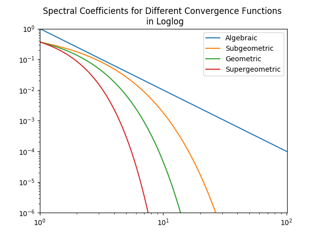
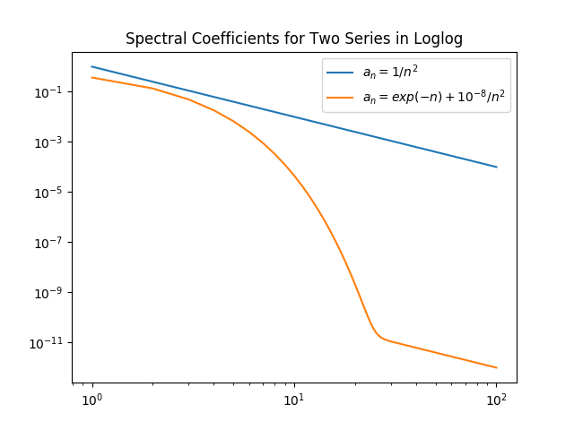
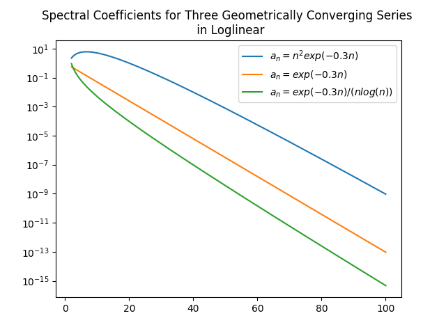
Figures from J. P. Boyd, *Chebyshev and Fourier Spectral Methods*, 2nd ed., Dover, New York, 2001.
Review Questions
- See this review link
Links to other resources
ChangeLog
- 2020-04-25 Mariana Silva mfsilva@illinois.edu: small text revisions
- 2020-02-19 Peter Sentz sentz2@illinois.edu: Add section on role of constants, change Big-Oh’s to “mathcal”
- 2020-01-26 Wanjun Jiang wjiang24@illinois.edu: add scientific notations, digits and figures
- 2018-01-31 Aming Ni amingni2@illinois.edu: changed three graphs
- 2018-01-16 Yu Meng yumeng5@illinois.edu: minor fixes throughout
- 2017-11-02 Erin Carrier ecarrie2@illinois.edu: adds changelog
- 2017-10-26 Erin Carrier ecarrie2@illinois.edu: adds review questions, minor changes throughout to better match termiology in class notes
- 2017-10-23 John Doherty jjdoher2@illinois.edu: first complete draft
- 2017-10-17 Luke Olson lukeo@illinois.edu: outline