Errors and Complexity
Learning objectives
- Compare and contrast relative and absolute error
- Categorize a cost as \(O(n^p)\)
- Categorize an error \(O(h^p)\)
- Identify algebraic vs exponential growth and convergence
Links and other content
- Lecture on Error, Accuracy and Convergence
- Chebyshev and Fourier Spectral Methods: Second Revised Edition
- Big-O Notation
Absolute and Relative Error
Results computed using numerical methods are inaccurate -- they are approximations to the true values. We can represent an approximate result as a combination of the true value and some error: \[ \text{Approximate Result} = \text{True Value} + \text{Error} \] \[ \hat{x} = x_0 + \Delta x \]
Given this problem setup we can define the absolute error as:
\[ \begin{equation} \text{Absolute Error} = |x_0 - \hat{x}| \end{equation} .\] This tells us how close our approximate result is to the actual answer. However, absolute error can become an unsatisfactory and misleading representation of the error depending on the magnitude of \(x_0\).
| Case 1 | Case 2 |
|---|---|
| \(x_0 = 0.1\), \(\hat{x} = 0.2\) | \(x_0 = 100.0\), \(\hat{x} = 100.1\) |
| \(\mid x_0 - \hat{x} \mid = 0.1\) | \(\mid x_0 - \hat{x} \mid = 0.1\) |
In both of these cases, the absolute error is the same, 0.1. However, we would intuitively consider case 2 more accurate than case 1 since our approximation is double the true value in case 1. Because of this, we define the relative error, which will be an error estimate independent of the magnitude. To obtain this we simply divide the absolute error by the absolute value of the true value.
\[ \begin{equation} \text{Relative Error} = \frac{|x_0 - \hat{x}|}{|x_0|} \end{equation} \]
If we consider the two cases again, we can see that the relative error will be much lower in the second case.
| Case 1 | Case 2 |
|---|---|
| \(x_0 = 0.1\), \(\hat{x} = 0.2\) | \(x_0 = 100.0\), \(\hat{x} = 100.1\) |
| \(\frac{\mid x_0 - \hat{x} \mid}{\mid x_0 \mid} = 1\) | \(\frac{\mid x_0 - \hat{x} \mid}{\mid x_0 \mid} = 10^{-3}\) |
Absolute and Relative Error of Vectors
If our calculated quanties are vectors then instead of using the absolute value function, we can use the norm instead. Thus, our formulas become \[ \begin{equation} \text{Absolute Error} = \|\mathbf{x} - \mathbf{\hat{x}}\| \end{equation} \]
\[ \begin{equation} \text{Relative Error} = \frac{\|\mathbf{x} - \mathbf{\hat{x}}\|}{\|\mathbf{x}\|} \end{equation} \]
We take the norm of the difference (and not the difference of the norms), because we are interested in how far apart these two quantites are. This formula is similar to finding that difference then using the vector norm to find the length of that difference vector.
Truncation Error vs. Rounding Error
Rounding error is the error that occurs from rounding values in a computation. This occurs constantly since computers use finite precision. If a number has \(n\) accurate digits, then that means the relative error of the approximation is \(\leq 10^{-n + 1}\).
Truncation error is the error from using an approximate algorithm in place of an exact mathematical procedure or function. For example, in the case of evaluating functions, we may represent our function by a finite taylor series up to degree \(n\). The truncation error is the error that is incurred by not using the \(n+1\) term and above.
Big-O Notation
Big-O notation is used to understand and describe asymptotic behavior. The definition in the cases of approching 0 or \(\infty\) are as follows:
Let \(f\) and \(g\) be two functions. Then \(f(x) = O(g(x))\) as \(x \rightarrow \infty\) if and only if there exists a value \(M\) and some \(x_0\) such that \(|f(x)| \leq M|g(x)|\) \(\forall x\) where \(x\geq x_0\)
Let \(f\) and \(g\) be two functions. Then \(f(h) = O(g(h))\) as \(h \rightarrow 0\) if and only if there exists a value \(M\) and some \(h_0\) such that \(|f(h)| \leq M|g(h)|\) \(\forall h\) where \(0 < h < h_0\)
But what if we want to consider the function approaching an arbitrary value? Then we can redefine the expression as:
Let \(f\) and \(g\) be two functions. Then \(f(x) = O(g(x))\) as \(x \rightarrow a\) if and only if there exists a value \(M\) and some \(\delta\) such that \(|f(x)| \leq M|g(x)|\) \(\forall x\) where \(0 < |x − a| < \delta\)
Big-O Examples
We can use Big-O to describe the time complexity of our algorithms.
Consider the case of matrix-matrix multiplication. If the size of each of our matrices is \(n \times n\), then the time it will take to multiply the matrices is \(O(n^3)\) meaning that \(\text{Run time} \approx C \cdot n^3\). Suppose we know that for \(n_1=1000\), the matrix-matrix multiplication takes 5 seconds. Estimate how much time it would take if we double the size of our matrices to \(2n \times 2n\).
We know that
\[\begin{align*} \text{Time}(2n_1) &\approx C \cdot (2n_1)^3 \\ &= C \cdot 2^3 \cdot n_1^3\\ &= 8 \cdot (C \cdot n_1^3) \\ &= 8 \cdot \text{Time}(n_1) \\ &= 40 \text{ seconds} \end{align*}\]
So, when we double the size of our our matrices to \(2n \times 2n\), the time becomes \((2n)^3 = 8n^3\). Thus, the runtime will be roughly 8 times as long.
A numerical method is called \(n\)-th order accurate if its truncation error \(E(h)\) obeys \(E(h) = O(h^n)\).
Consider solving an interpolation problem. We have an interval of length \(h\) where our interpolant is valid and we know that our approximation is order \(O(h^2)\). What this means is that as we decrease h, our interval length, our error will decrease quadratically. Using the definition of Big-O, we know that \(\text{Error} = C \cdot h^2\) where \(C\) is some constant.
Convergence Definitions
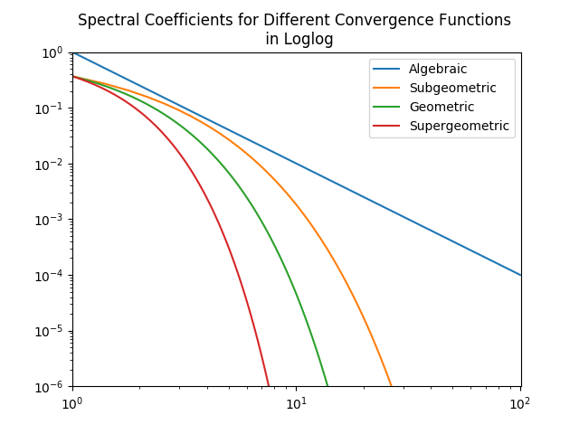
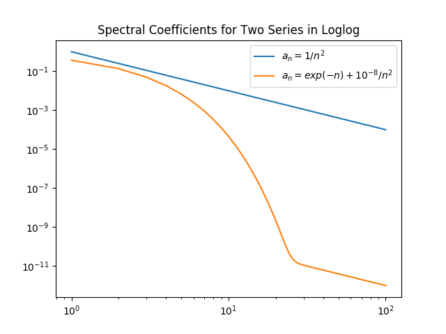
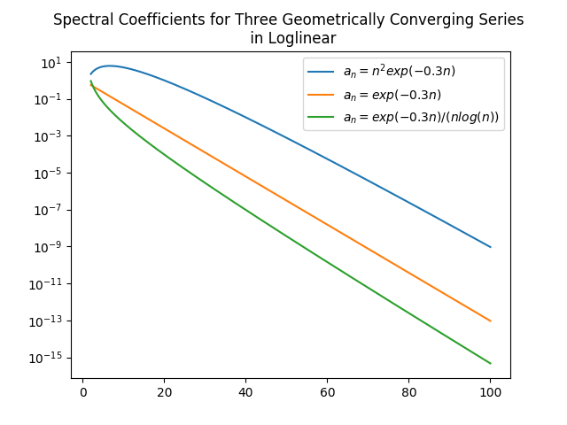
Algebraic growth/convergence is when the coefficients \(a_n\) in the sequence we are interested in behave like \(O(n^{\alpha})\) for growth and \(O(1/n^{\alpha})\) for convergence, where \(\alpha\) is called the algebraic index of convergence. A sequence that grows or converges algebraically is a straight line in a log-log plot.
Exponential growth/convergence is when the coefficients \(a_n\) of the sequence we are interested in behave like \(O(e^{qn^{\beta}})\) for growth and \(O(e^{-qn^{\beta}})\) for convergence, where \(q\) is a constant for some \(\beta > 0\). Exponential growth is much faster than algebraic growth. Exponential growth/convergence is also sometimes called spectral growth/convergence. A sequence that grows exponentially is a straight line in a log-linear plot. Exponential convergence is often further classified as supergeometric, geometric, or subgeometric convergence.
The figures below, taken from
J. P. Boyd, Chebyshev and Fourier Spectral Methods, 2nd ed., Dover, New York, 2001.
(link under "Links and other content"), illustrate examples of algebraic and exponential convergence.
Review Questions
- What is the formula for relative error?
- What is the formula for absolute error?
- Which is usually the better way to calculate error?
- If you have k accurate significant digits, what is the tightest bound on your relative error?
- Given a maximum relative error, what is the largest (or smallest) value you could have?
- How do you compute relative and absolute error for vectors?
- What is truncation error?
- What is rounding error?
- What does it mean for an algorithm to take O(n^3) time?
- Can you give an example of an operation that takes O(n^2) time?
- What does it mean for error to follow O(h^4)?
- Can you simplify O(h^5 + h^2 + h)? What assumption do you need to make?
- If you know an operation is O(n^4), can you predict its time/error on unseen inputs from inputs that you already have?
- If you are given runtime or error data for an operation, can you find the best x such that the operation is O(n^x)?
- What is algebraic growth/convergence?
- What is exponential growth/convergence?
ChangeLog
- 2018-01-16 Yu Meng yumeng5@illinois.edu: minor fixes throughout
- 2017-11-02 Erin Carrier ecarrie2@illinois.edu: adds changelog
- 2017-10-26 Erin Carrier ecarrie2@illinois.edu: adds review questions, minor changes throughout to better match termiology in class notes
- 2017-10-23 John Doherty jjdoher2@illinois.edu: first complete draft
- 2017-10-17 Luke Olson lukeo@illinois.edu: outline