Singular Value Decompositions
Learning Objectives
- Construct an SVD of a matrix
- Identify pieces of an SVD
- Use an SVD to solve a problem
Links and Other Content
Nothing here yet.
Singular Value Decomposition
An \(m \times n\) real matrix \(A\) has a singular value decomposition of the form \[ A = U \Sigma V^\top, \] where
- \(U\) is an \(m \times m\) orthogonal matrix whose columns are eigenvectors of \(A A^\top\). The columns of \(U\) are called the left singular vectors of \(A\).
- \(\Sigma\) is an \(m \times n\) diagonal matrix of the form: \[ \Sigma = \begin{bmatrix} \sigma_1 & & \\ & \ddots & \\ & & \sigma_n \\ 0 & & 0 \\ \vdots & \ddots & \vdots \\ 0 & & 0 \end{bmatrix}, \] where \(\sigma_1 \ge \sigma_2 \dots \ge \sigma_n \ge 0\) are the square roots of the eigenvalues values of \(A^\top A\). The diagonal entries are called the singular values of \(A\).
- \(V\) is an \(n \times n\) orthogonal matrix whose columns are eigenvectors of \(A^\top A\) The columns of \(V\) are called the right singular vectors of \(A\).
Note: The time-complexity for computing the SVD factorization of an arbitary \(m \times n\) matrix is \(O(m^2n + n^3)\).
Example: Computing the SVD
We begin with the following non-square matrix, \(A\): \[ A = \left[ \begin{array}{ccc} 3 & 2 & 3 \\ 8 & 8 & 2 \\ 8 & 7 & 4 \\ 1 & 8 & 7 \\ 6 & 4 & 7 \\ \end{array} \right]. \]
Compute \(A^\top A\): \[ A^\top A = \left[ \begin{array}{ccc} 174 & 158 & 106 \\ 158 & 197 & 134 \\ 106 & 134 & 127 \\ \end{array} \right]. \]
Compute the eigenvectors and eigenvalues of \(A^\top A\): \[ \lambda_1 = 437.479, \quad \lambda_2 = 42.6444, \quad \lambda_3 = 17.8766, \\ \boldsymbol{v}_1 = \begin{bmatrix} 0.585051 \\ 0.652648 \\ 0.481418\end{bmatrix}, \quad \boldsymbol{v}_2 = \begin{bmatrix} -0.710399 \\ 0.126068 \\ 0.692415 \end{bmatrix}, \quad \boldsymbol{v}_3 = \begin{bmatrix} 0.391212 \\ -0.747098 \\ 0.537398 \end{bmatrix}. \]
Construct \(V\) from the eigenvectors of \(A^\top A\): \[ V = \left[ \begin{array}{ccc} 0.585051 & -0.710399 & 0.391212 \\ 0.652648 & 0.126068 & -0.747098 \\ 0.481418 & 0.692415 & 0.537398 \\ \end{array} \right]. \]
Construct \(\Sigma\) from the square roots of the eigenvalues of \(A^\top A\): \[ \Sigma = \begin{bmatrix} 20.916 & 0 & 0 \\ 0 & 6.53207 & 0 \\ 0 & 0 & 4.22807 \end{bmatrix} \]
Find \(U\) by solving \(U\Sigma = AV\). For our simple case, we can find \(U = AV\Sigma^{-1}\). You could also find \(U\) by computing the eigenvectors of \(AA^\top\). \[ U = \overbrace{\left[ \begin{array}{ccc} 3 & 2 & 3 \\ 8 & 8 & 2 \\ 8 & 7 & 4 \\ 1 & 8 & 7 \\ 6 & 4 & 7 \\ \end{array} \right]}^{A} \overbrace{\left[ \begin{array}{ccc} 0.585051 & -0.710399 & 0.391212 \\ 0.652648 & 0.126068 & -0.747098 \\ 0.481418 & 0.692415 & 0.537398 \\ \end{array} \right]}^{V} \overbrace{\left[ \begin{array}{ccc} 0.047810 & 0.0 & 0.0 \\ 0.0 & 0.153133 & 0.0 \\ 0.0 & 0.0 & 0.236515 \\ \end{array} \right]}^{\Sigma^{-1}} \\ U = \left[ \begin{array}{ccc} 0.215371 & 0.030348 & 0.305490 \\ 0.519432 & -0.503779 & -0.419173 \\ 0.534262 & -0.311021 & 0.011730 \\ 0.438715 & 0.787878 & -0.431352\\ 0.453759 & 0.166729 & 0.738082\\ \end{array} \right] \]
We obtain the following singular value decomposition for \(A\): \[ \overbrace{\left[ \begin{array}{ccc} 3 & 2 & 3 \\ 8 & 8 & 2 \\ 8 & 7 & 4 \\ 1 & 8 & 7 \\ 6 & 4 & 7 \\ \end{array} \right]}^{A} = \overbrace{\left[ \begin{array}{ccc} 0.215371 & 0.030348 & 0.305490 \\ 0.519432 & -0.503779 & -0.419173 \\ 0.534262 & -0.311021 & 0.011730 \\ 0.438715 & 0.787878 & -0.431352\\ 0.453759 & 0.166729 & 0.738082\\ \end{array} \right]}^{U} \overbrace{\left[ \begin{array}{ccc} 20.916 & 0 & 0 \\ 0 & 6.53207 & 0 \\ 0 & 0 & 4.22807 \\ \end{array} \right]}^{\Sigma} \overbrace{\left[ \begin{array}{ccc} 0.585051 & 0.652648 & 0.481418 \\ -0.710399 & 0.126068 & 0.692415\\ 0.391212 & -0.747098 & 0.537398\\ \end{array} \right]}^{V^\top} \]
Note: We computed the reduced SVD factorization (i.e. \(\Sigma\) is square, \(U\) is non-square) here.
SVD: Solving the Least Squares Problem
Given the following linear equation \[ A \boldsymbol{x} \cong \boldsymbol{b}, \] where \(A\) is a non-square matrix whose SVD factorization (\(A = U\Sigma V^\top\)) is known, we can compute the solution which minimizes the sum of squared differences as: \[ \boldsymbol{x} = V\Sigma^{+}U^\top\boldsymbol{b}, \] where \(\Sigma^{+}\) is the pseudoinverse of the singular matrix computed by taking the reciprocal of the non-zero diagonal entries, leaving the zeros in place and transposing the resulting matrix. For example: \[ \Sigma = \begin{bmatrix} \sigma_1 & & \\ & \ddots & \\ & & \sigma_n \\ 0 & & 0 \\ \vdots & \ddots & \vdots \\ 0 & & 0 \end{bmatrix} \quad \implies \quad \Sigma^{+} = \begin{bmatrix} \frac{1}{\sigma_1} & & & 0 & \dots & 0 \\ & \ddots & & & \ddots &\\ & & \frac{1}{\sigma_n} & 0 & \dots & 0 \\ \end{bmatrix}. \]
Note: Solving the least squares problem has a time complexity of \(O(\max\{m^2, n^2\})\) for a known full SVD factorization, and \(O(mn)\) for a known reduced SVD factorization.
(Moore-Penrose) Pseudoinverse
Given a non-square matrix \(A\) whose SVD factorization (\(A = U\Sigma V^\top\)) is known, the pseudoinverse of \(A\) is defined as: \[ A^{+} = V\Sigma^{+}U^\top \]
Reduced SVD
The SVD factorization of a non-square matrix \(A\) of size \(m \times n\) can be reprsented in a compact fashion:
- For \(m \ge n\): \(U\) is \(m \times n\), \(\Sigma\) is \(n \times n\), and \(V\) is \(n \times n\)
- For \(m \le n\): \(U\) is \(m \times m\), \(\Sigma\) is \(m \times m\), and \(V\) is \(n \times m\) (note if \(V\) is \(n \times m\), then \(V^\top\) is \(m \times n\))
The following figure depicts the reduced SVD factorization (in red) against the full SVD factorizations (in gray).

2-Norm based on Singular Values
The induced 2-norm of a matrix, \(A\), is given by its largest singular value: \[ \|A\|_2 = \max_{\|y\| = 1} \|\Sigma y\|_2 = \sigma_1, \] where \(\Sigma\) is the diagonal matrix of singular values of \(A\).
Example: 2-Norm based on Singular Values
We begin with the following non-square matrix, \(A\): \[ A = \left[ \begin{array}{ccc} 3 & 2 & 3 \\ 8 & 8 & 2 \\ 8 & 7 & 4 \\ 1 & 8 & 7 \\ 6 & 4 & 7 \\ \end{array} \right]. \]
The matrix of singular values, \(\Sigma\), computed from the SVD factorization is: \[ \Sigma = \left[ \begin{array}{ccc} 20.916 & 0 & 0 \\ 0 & 6.53207 & 0 \\ 0 & 0 & 4.22807 \\ \end{array} \right]. \]
Following our definition, we have the 2-norm of \(A\) as \[ \|A\|_2 = 20.916.\]
Computing 2-Norm Condition Number from Singular Values
The 2-norm condition number of a matrix \(A\) is given by the ratio of its largest singular value to its smallest singular value: \[\text{cond}_2(A) = \|A\|_2 \|A^{-1}\|_2 = \sigma_{\max}/\sigma_{\min}.\] If \(\text{rank}(A) < \min(m,n)\), then \(\sigma_{\min} = 0\) so \(\text{cond}_2(A) = \infty\).
Low-rank Approximation
The best rank-\(k\) approximation for a \(m \times n\) matrix \(A\), (where, \(k \le m\) and \(k \le n\)) for some matrix norm \(\| \cdot \|\) is one that minimizes the following problem: \[ \begin{aligned} &\min_{A_k} \ \|A - A_k\| \\ &\textrm{such that} \quad \mathrm{rank}(A_k) \le k. \end{aligned} \]
Under the induced \(2\)-norm, the best rank-\(k\) approximation is given by the sum of the first \(k\) outer products of the left and right singular vectors scaled by the corresponding singular value (where, \(\sigma_1 \ge \dots \ge \sigma_n\)): \[ A_k = \sigma_1 \boldsymbol{u}_1 \boldsymbol{v}_1^\top + \dots \sigma_k \boldsymbol{u}_k \boldsymbol{v}_k^\top \]
Observe that the norm of the difference between the best approximation and the matrix under the induced \(2\)-norm condition is the magnitude of the \((k+1)^\text{th}\) singular value of the matrix: \[ \|A - A_k\|_2 = \left|\left|\sum_{i=k+1}^n \sigma_i \boldsymbol{u}_i \boldsymbol{v}_i^\top\right|\right|_2 = \sigma_{k+1} \]
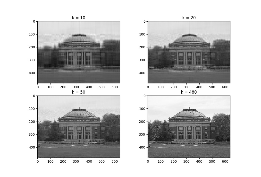
Example: Low-rank Approximation
The following code snippet performs best rank-\(k\) approximation (under \(2\)-norm assumptions) on an image:
import numpy as np

def bestk(A, k):
  U,S,V = np.linalg.svd(A, full_matrices=False)
  return U[:, :k] @ np.diag(S[:k]) @ V[:k, :]

from urllib.request import urlopen
from scipy.misc import imread
import matplotlib.pyplot as plt

url = 'https://upload.wikimedia.org/wikipedia/en/thumb/a/a8/Foellinger_Auditorium.jpg/640px-Foellinger_Auditorium.jpg'

with urlopen(url) as img:
  foellinger = imread(img, mode='F')
  low_10 = bestk(foellinger, 10)
  low_20 = bestk(foellinger, 20)
  low_50 = bestk(foellinger, 50)

  plt.subplot(2, 2, 1)
  plt.imshow(low_10, cmap='gray')
  plt.title("k = 10")
  plt.subplot(2, 2, 2)
  plt.imshow(low_20, cmap='gray')
  plt.title("k = 20")
  plt.subplot(2, 2, 3)
  plt.imshow(low_50, cmap='gray')
  plt.title("k = 50")
  plt.subplot(2, 2, 4)
  plt.imshow(foellinger, cmap='gray')
  plt.title("k = 480")
  plt.show()
Review Questions
- For a matrix \(A\) with SVD decomposition \(A = U \Sigma V^\top\), what are the columns of \(U\) and how can we find them? What are the columns of \(V\) and how can we find them? What are the entries of \(\Sigma\) and how can we find them?
- What special properties are true of \(U\)? \(V\)? \(\Sigma\)?
- What are the shapes of \(U\), \(\Sigma\), and \(V\) in the full SVD of an \(m \times n\) matrix?
- What are the shapes of \(U\), \(\Sigma\), and \(V\) in the reduced SVD of an \(m \times n\) matrix?
- What is the cost of computing the SVD?
- Given an already computed SVD of a matrix \(A\), what is the cost of using the SVD to solve a linear system \(A\boldsymbol{x} = \boldsymbol{b}\)? How would you use the SVD to solve this system?
- Given an already computed SVD of a matrix \(A\), what is the cost of using the SVD to solve a least squares problem \(A \boldsymbol{x} \cong \boldsymbol{b}\)? How do you solve a least squares problem using the SVD?
- How do you use the SVD to compute a low-rank approximation of a matrix? For a small matrix, you should be able to compute a given low rank approximation (i.e. rank-one, rank-two).
- Given the SVD of a matrix \(A\), what is the SVD of \(A^{+}\) (the psuedoinverse of \(A\))?
- Given the SVD of a matrix \(A\), what is the 2-norm of the matrix? What is the 2-norm condition number of the matrix?
ChangeLog
- 2017-12-04 Arun Lakshmanan : fix best rank approx, svd image
- 2017-11-15 Erin Carrier : adds review questions, adds cond num sec, removes normal equations, minor corrections and clarifications
- 2017-11-13 Arun Lakshmanan : first complete draft
- 2017-10-17 Luke Olson : outline