Optimization
Learning Objectives
- Set up a problem as an optimization problem
- Use a method to find an approximation of the minimum
- Identify challenges in optimization
Links and Other Content
- None here yet
Minima of a Function
Consider a function \(f:\;S\to \mathbb{R}\), and \(S\subset\mathbb{R}^n\). The point \(\boldsymbol{x}^*\in S\) is called the minimizer or minimum of \(f\) if \(f(\boldsymbol{x}^*)\leq f(\boldsymbol{x}) \, \forall x\in S\).
For the rest of this topic we try to find the minimizer of a function, as one can easily find the maximizer of a function \(f\) by trying to find the minimizer of \(-f\).
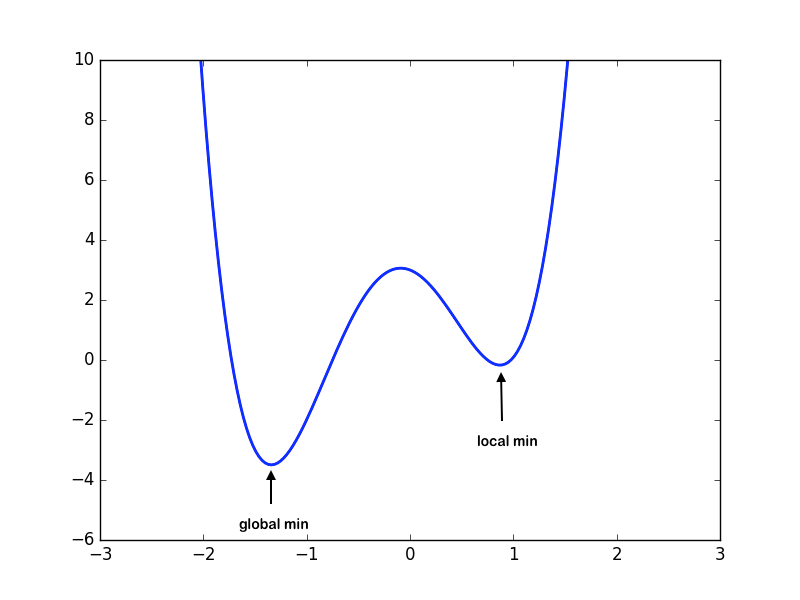
Local vs. Global Minima
Consider a domain \(S\subset\mathbb{R}^n\), and \(f:S\to\mathbb{R}\).
Local Minima: \(\boldsymbol{x}^*\) is a local minimum if \(f(\boldsymbol{x}^*)\leq f(\boldsymbol{x})\) for all feasible \(\boldsymbol{x}\) in some neighborhood of \(\boldsymbol{x}^*\).
Global Minima: \(\boldsymbol{x}^*\) is a global minimum if \(f(\boldsymbol{x}^*)\leq f(\boldsymbol{x})\) for all \(\boldsymbol{x}\in S\).
It might to interesting to note that it is easier to find the local minimum than the global minimum. Given a function, finding whether a global minimum exists over the domain is in itself a non-trivial problem. Hence, we will limit ourselves to finding the local minima of the function.
Recall: Criteria for 1-D Local Minima
In the case of 1-D optimization, we can tell if a point \(x^* \in S\) is a local minimum by considering the values of the derivatives. Specifically,
- Necessary condition: \(f'(x^*) = 0\)
- Sufficient condition: \(f'(x^*) = 0\) and \(f''(x^*) > 0\).
Example: Consider the function \[f(x) = x^3 - 6x^2 + 9x -6\] The first and second derivatives are as follows: \[f'(x) = 3x^2-12x+9\\ f''(x) = 6x-12\]
The critical points are tabulated as:
| \(\boldsymbol{x}\) | \(\boldsymbol{f'(x)}\) | \(\boldsymbol{f''(x)}\) | Characteristic |
|---|---|---|---|
| 3 | 0 | \(6\) | Local Minimum |
| 1 | 0 | \(-6\) | Local Maximum |
Looking at the table, we see that \(x=3\) satisfies the sufficient condition for being a local minimum.
Criteria for \(n\)-D Local Minima
As we saw in 1-D, on extending that concept to \(n\) dimensions we can tell if \(\boldsymbol{x}^*\) is a local minimum by the following conditions:
- Necessary condition: the gradient \(\nabla f(\boldsymbol{x}^*) = \boldsymbol{0}\)
- Sufficient condition: the gradient \(\nabla f(\boldsymbol{x}^*) = \boldsymbol{0}\) and the Hessian matrix \(H_f(\boldsymbol{x^*})\) is positive definite.
Definiton of Gradient and Hessian Matrix
Given \(f:\mathbb{R}^n\to \mathbb{R}\) we define the gradient function \(\nabla f: \mathbb{R}^n\to\mathbb{R}^n\) as: \[ \nabla f(\boldsymbol{x}) = \begin{pmatrix} \frac{\partial f}{\partial x_1}\\ \frac{\partial f}{\partial x_2}\\ \vdots\\ \frac{\partial f}{\partial x_n} \end{pmatrix} \]
Given \(f:\mathbb{R}^n\to \mathbb{R}\) we define the Hessian matrix \(H_f: \mathbb{R}^n\to\mathbb{R}^{n\times n}\) as:
\[H_f(\boldsymbol{x}) = \begin{bmatrix} \frac{\partial^2 f}{\partial x_1^2} & \frac{\partial f}{\partial x_1\partial x_2} & \ldots & \frac{\partial f}{\partial x_1\partial x_n} \\ \frac{\partial^2 f}{\partial x_2\partial x_1} & \frac{\partial f}{\partial x_2^2} & \ldots & \frac{\partial f}{\partial x_2\partial x_n} \\ \vdots & \vdots & \ddots & \vdots \\ \frac{\partial^2 f}{\partial x_n\partial x_1} & \frac{\partial f}{\partial x_n\partial x_2} & \ldots & \frac{\partial f}{\partial x_n^2} \end{bmatrix}\]
Unimodal Function
A 1-dimensional function \(f: S\to\mathbb{R}\), is said to be unimodal if for all \(x_1, x_2 \in S\), with \(x_1<x_2\) and \(x^*\) as the minimizer:
- If \(x_2 < x^*\Rightarrow f(x_1)>f(x_2)\)
- If \(x^* < x_1\Rightarrow f(x_1)<f(x_2)\)
In order to simplify, we will consider our objective function to be unimodal as it guarantees us a unique solution to the minimization problem.
Optimization Techniques in 1-D
Newton's Method
We know that in order to find a local minimum we need to find the root of the derivative of the function. Inspired from Newton's method for root-finding we define our iterative scheme as follows: \[x_{k+1} = x_k - \frac{f'(x_k)}{f''(x_k)}\] This is equivalent to using Newton's method for root finding to solve \(f'(x) = 0\), so the method converges quadratically, provided that \(x_k\) is sufficiently close to the local minimum.
For Newton's method for optimization in 1-D, we evaluate \(f'(x_k)\) and \(f''(x_k)\), so it requires 2 function evaluations per iteration.
Golden Section Search
Inspired by bisection for root finding, we define an interval reduction method for finding the minimum of a function. As in bisection where we reduce the interval such that the reduced interval always contains the root, in Golden Section Search we reduce our interval such that it always has a unique minimizer in our domain.
Algorithm to find the minima of \(f: [a, b] \to \mathbb{R}\):
Our goal is to reduce the domain to \([x_1, x_2]\) such that:
- If \(f(x_1) > f(x_2)\) our new interval would be \((x_1, b)\)
- If \(f(x_1) \leq f(x_2)\) our new interval would be \((a, x_2)\)
We select \(x_1, x_2\) as interior points to \([x_1, x_2]\) by choosing a \(0\leq\tau\leq 1\) and setting:
- \(x_1 = a + (1-\tau)(b-a)\)
- \(x_2 = a + \tau(b-a)\)
The challenging part is to select a \(\tau\) such that we ensure symmetry i.e. after each iteration we reduce the interval by the same factor, which gives us the indentity \(\tau^2 = 1-\tau\). Hence,
\[\tau = \frac{\sqrt{5}-1}{2}.\]
As the interval gets reduced by a fixed factor each time, it can be observed that the method is linearly convergent. The number \(\frac{\sqrt{5}-1}{2}\) is the inverse of the "Golden-Ratio" and hence this algorithm is named Golden Section Search.
In golden section search, we do not need to evaluate any derivatives of \(f(x)\). At each iteration we need \(f(x_1)\) and \(f(x_2)\), but one of \(x_1\) or \(x_2\) will be the same as the previous iteration, so it only requires 1 additional function evaluation per iteration (after the first iteration).
Optimization in \(n\) Dimensions
Steepest Descent
The negative of the gradient of a differentiable function \(f: \mathbb{R}^n\to\mathbb{R}\) points downhill i.e. towards points in the domain having lower values. This hints us to move in the direction of \(-\nabla f\) while searching for the minimum until we reach the point where \(\nabla f(\boldsymbol{x}) = \boldsymbol{0}\). Therefore, at a point \(\boldsymbol{x}\) the direction ''\(-\nabla f(\boldsymbol{x})\)'' is called the direction of steepest descent.
Hence, we know the direction we need to move to approach the minimum but we still do not know the distance we need to move in order to approach the minimum. If \(\boldsymbol{x_k}\) was our earlier point then we select the next guess by moving it in the direction of the negative gradient: \[\boldsymbol{x_{k+1}} = \boldsymbol{x_k} + \alpha(-\nabla f(\boldsymbol{x_k})).\]
The next problem would be to find the \(\alpha\), and we use the 1-dimensional optimization algorithms to find the required \(\alpha\). Hence, the problem translates to: \[ \boldsymbol{s} = -\nabla f(\boldsymbol{x_k}) \\ \min_{\alpha}\left( f\left(\boldsymbol{x_k} + \alpha \boldsymbol{s}\right)\right) \]
The steepest descent algorithm can be summed up in the following function:
import numpy.linalg as la
import scipy.optimize as opt
import numpy as np

def obj_func(alpha, x, s):
    # code for computing the objective function at (x+alpha*s)
    return f_of_x_plus_alpha_s

def gradient(x):
    # code for computing gradient
    return grad_x

def steepest_descent(x_init):
    x_new = x_init
    x_prev = np.random.randn(x_init.shape[0])
    while(la.norm(x_prev - x_new) > 1e-6):
        x_prev = x_new
        s = -gradient(x_prev)
        alpha = opt.minimize_scalar(obj_func, args=(x_prev, s)).x
        x_new = x_prev + alpha*s

    return x_new
The steepest descent method converges linearly.
Newton's Method
Newton's Method in \(n\) dimensions is similar to Newton's method for root finding in \(n\) dimensions, except we just replace the \(n\)-dimensional function by the gradient and the Jacobian matrix by the Hessian matrix. We can arrive at the result by considering the Taylor expansion of the function. \[ f(\boldsymbol{x}+s) \approx f(\boldsymbol{x}) + \nabla f(\boldsymbol{x})^Ts + \frac{1}{2}s^TH_f(\boldsymbol{x})s \] We solve for \(\nabla f(\boldsymbol{s}) = \boldsymbol{0}\) for \(\boldsymbol{s}\). So, the equation can be translated as: \[H_f(\boldsymbol{x})\boldsymbol{s} = -\nabla f(\boldsymbol{x}).\] The Newton's Method can be expressed as a python function as follows:
import numpy as np
def hessian(x):
    # Computes the hessian matrix corresponding the given objective function
    return hessian_matrix_at_x

def gradient(x):
    # Computes the gradient vector corresponding the given objective function
    return gradient_vector_at_x

def newtons_method(x_init):
    x_new = x_init
    x_prev = np.random.randn(x_init.shape[0])
    while(la.norm(x_prev-x_new)>1e-6):
        x_prev = x_new
        s = -la.solve(hessian(x_prev), gradient(x_prev))
        x_new = x_prev + s
    return x_new
Review Questions
- What are the necessary and sufficient conditions for a point to be a local minimum in one dimension?
- What are the necessary and sufficient conditions for a point to be a local minimum in \(n\) dimensions?
- How do you classify extrema as minima, maxima, or saddle points?
- What is the difference between a local and a global minimum?
- What does it mean for a function to be unimodal?
- What special attribute does a function need to have for golden section search to find a minimum?
- Run one iteration of golden section search.
- Calculate the gradient of a function (function has many inputs, one output).
- Calculate the Jacobian of a function (function has many inputs, many outputs).
- Calculate the Hessian of a function.
- Find the search direction in steepest/gradient descent.
- Why must you perform a line search each step of gradient descent?
- Run one step of Newton's method in one dimension.
- Run one step of Newton's method in \(n\) dimensions.
- When does Newton's method fail to converge to a minimum?
- What operations do you need to perform each iteration of golden section search?
- What operations do you need to perform each iteration of Newton's method in one dimension?
- What operations do you need to perform each iteration of Newton's method in \(n\) dimensions?
- What is the convergence rate of Newton's method?
ChangeLog
- 2017-11-25 Adam Stewart adamjs5@illinois.edu: fixes missing partial in Hessian matrix
- 2017-11-20 Kaushik Kulkarni kgk2@illinois.edu: fixes table formatting
- 2017-11-20 Nate Bowman nlbowma2@illinois.edu: adds review questions
- 2017-11-20 Erin Carrier ecarrie2@illinois.edu: removes Gauss-Newton/LM, minor rewording and small changes throughout
- 2017-11-20 Kaushik Kulkarni kgk2@illinois.edu and Arun Lakshmanan lakshma2@illinois.edu: first full draft
- 2017-10-17 Luke Olson lukeo@illinois.edu: outline