import numpy as np
import numpy.linalg as la
import scipy.optimize as opt
import matplotlib.pyplot as plt
Steepest Descent in Machine Learning
Recall that steepest descent is an optimization algorithm that computes the minimum of a function by $$x_{k+1} = x_k - \alpha_k \nabla f(x_k),$$ where $x_k$ is the solution at step $k$, and $\alpha_k$ is a line search parameter that is computed by solving the 1-dimensional optimization problem $$ \alpha_k = \min_{\alpha_k} f(x_k - \alpha_k \nabla f(x_k)) $$
We will explore how we can use steepest descent in machine learning.
1) Example 1: Linear Regression
In this first example, we will use steepest descent to compute a linear regression (line of best fit) model over some data.
(This isn't the only way of computing the line of best fit and later on in the course we will explore other methods for accomplishing this same task.)
The data that we will be working with is an $n \times 2$ numpy array where each row represents an $(x_i,y_i)$ pair.
data = np.genfromtxt('data.csv', delimiter=',')
Plot the data to see what it looks like.
plt.scatter(data[:,0], data[:,1])
plt.xlabel('x')
plt.ylabel('y')
plt.show()
The first step in applying steepest descent is to formulate a function that we want to minimize.
To compute the line of best fit, we want to construct a line ($y = mx+b$) and minimize the error between this line and the data points. Therefore, we want to minimize the sum of square error: $$ E(m,b) = \frac{1}{N} \sum_{i=1}^N (y_i - (mx_i+b))^2 $$
that can be written as a unconstrained optimization problem:
$$\min_{m,b} E(m,b) $$
Since we will be using steepest descent to solve this optimization problem, we need to be able to evaluate $E$ and $\nabla E$.
a) Let's write a function to compute the error $E(m,b)$. The function will have the following signature:
def E(mb, data):
    # Compute error in the linear regression model using the sum of square error formula
    # mb: Numpy array of length 2 with first entry as m and second entry as b
    # data: 2D Numpy array of length nx2 where each row represents an (xi,yi) pair with n data points
    # totalError: Scalar output of sum of square error formula
    totalError = ...
    return totalError
You can try $m=1$ and $b=2$ as arguments to help debugging your code snippet. Your function should return 594.259213603709.
b) Now that we the function that we want to minimize, we need to compute it's gradient $\nabla E$.
You should compute the analytical form of these derivatives by hand (it is a good practice!) You can also later compare your results with SymPy. Note that the independent variables are m and b. The function should have the following signature:
def gradE(mb, data):
    # Compute the gradient of the error in the linear regression model
    # mb: Numpy array of length 2 with first entry as m and second entry as b
    # data: 2D Numpy array of length nx2 where each row represents an (xi,yi) pair with n data points

    # grad: Numpy array of length 2 with first entry as partial derivative with respect to m
    #       and second entry as partial derivative with respect to b
    m_gradient = ...
    b_gradient = ...
    grad = np.array([m_gradient, b_gradient])
    return grad
You can try $m=1$ and $b=2$ as arguments to help debugging your code snippet. Your function should return [-2192.94722958 -43.55341818].
mb = np.array([1.,2.])
print(gradE(mb,data))
The last thing that we need before we can write a function for steepest descent, is to solve a 1-dimensional optimization problem to solve for the line search parameter. However, in machine learning we want to avoid this and employ a heuristic approach.
Instead, we will pick a "learning rate" and use that instead of a line search parameter.
learning_rate = 0.0001
We should now have everything that we need to use steepest descent.
Steepest descent using a fixed learning rate
Let's write a function for steepest descent with the following signature:
def steepest_descent(mb, learning_rate, data, num_iterations):
    # mb: Numpy array of length 2 containing initial guess for parameters m and b
    # learning_rate: Scalar with the learning rate that will be applied to steepest descent
    # data: 2D Numpy array of length nx2 where each row represents an (xi,yi) pair with n data points
    # num_iterations: Integer with the number of iterations to run steepest descent
    # mb_list: list that contains the history of values [m,b] for each iteration
    return mb_list
Note that in the above, we are not imposing a tolerance as stopping criteria, but instead letting the algorithm iterates for a fixed number of steps (num_iterations).
Now, we have everything we need to compute a line of best fit for a given data set.
Let's assume that our initial guess for the linear regression model is 0, meaning that
m = 0.
b = 0.
Let's plot the data again but now with our model to see what the initial line of best fit looks like.
# Initial guess for m and b
mb_initial = np.array([0.,0.])

# Line y = mx + b
xs = np.linspace(20,70,num=1000)
ys = mb_initial[0]*xs + mb_initial[1]

plt.scatter(data[:,0], data[:,1], label = 'data')
plt.plot(xs,ys,'r', label = 'Initial model')
plt.legend()
plt.xlabel('x')
plt.ylabel('y')
plt.show()
Perform 100 iterations of steepest descent and plot the model (line) with the optimized values of $m$ and $b$.
Let's investigate the error in the model to see how steepest descent is minimizing the function.
Compute the error (using the function E) for each update of m and b that was stored as a return value in steepest_descent. Store the error for each iteration in the list errors. Note: you could have included this calculation inside your steepest_descent function.
Plot the error at each iteration.
errors = np.array(errors)
plt.semilogy(errors, label = 'error')
plt.xlabel('iteration')
plt.legend()
plt.show()
It looks like the algorithm didn't need all the 100 iterations. Can you think of a better stopping criteria? Try that later (for now, let's just move on to the next section).
Steepest descent - what happens when we change the learning rate?
For all these experiments, we stated that learning_rate $= 0.0001$. What would happen if we were to increase or decrease the learning rate?
Run the steps above for the learning rates [1e-6, 1e-5, 1e-4]. Save the values of m and b obtained for the three different learning rates.
1) Plot the data and the model (lines) for the three different values of learning_rate
2) Plot the error for the three different values of learning_rate
As we can see from the above plots, the number of steps for convergence will change depending on the learning_rate.
Steepest descent using golden-section search
In class, we learned about golden-section search for solving for the line search parameter. How can we use it to compute the parameter $\alpha$ in steepest descent for this example?
We need to first create a wrapper function so that we can minimize $f(x_k - \alpha \nabla f(x_k))$ with respect to $\alpha$.
def objective_1d(alpha, mb, data):
    mb_next = mb - alpha * gradE(mb, data)
    return E(mb_next, data)
Create a new steepest descent function to compute the line search parameter. Use scipy.optimize.golden to compute $\alpha$.
alpha = opt.golden(objective_1d, args = (mb,data))
The steepest descent function signature should be:
def steepest_descent_gss(mb, data, num_iterations):
    # mb: Numpy array of length 2 containing initial guess for parameters m and b
    # data: 2D Numpy array of length nx2 where each row represents an (xi,yi) pair with n data points
    # num_iterations: Integer with the number of iterations to run steepest descent
    # mb_list: list that contains the history of values [m,b] for each iteration
    return mb_list
Plot the error of using golden-section search for the line search parameter and compare the results with using a learning rate. Does this improve the convergence? How many iterations does it take for steepest descent to converge?
In practice, we don't use golden-section search in machine learning and instead we employ the heuristic that we described earlier of using a learning rate (note that the learning rate is not fixed, but updated using different methods). Why would we want use a learning rate over a line search parameter?
Example 2: Location of Cities
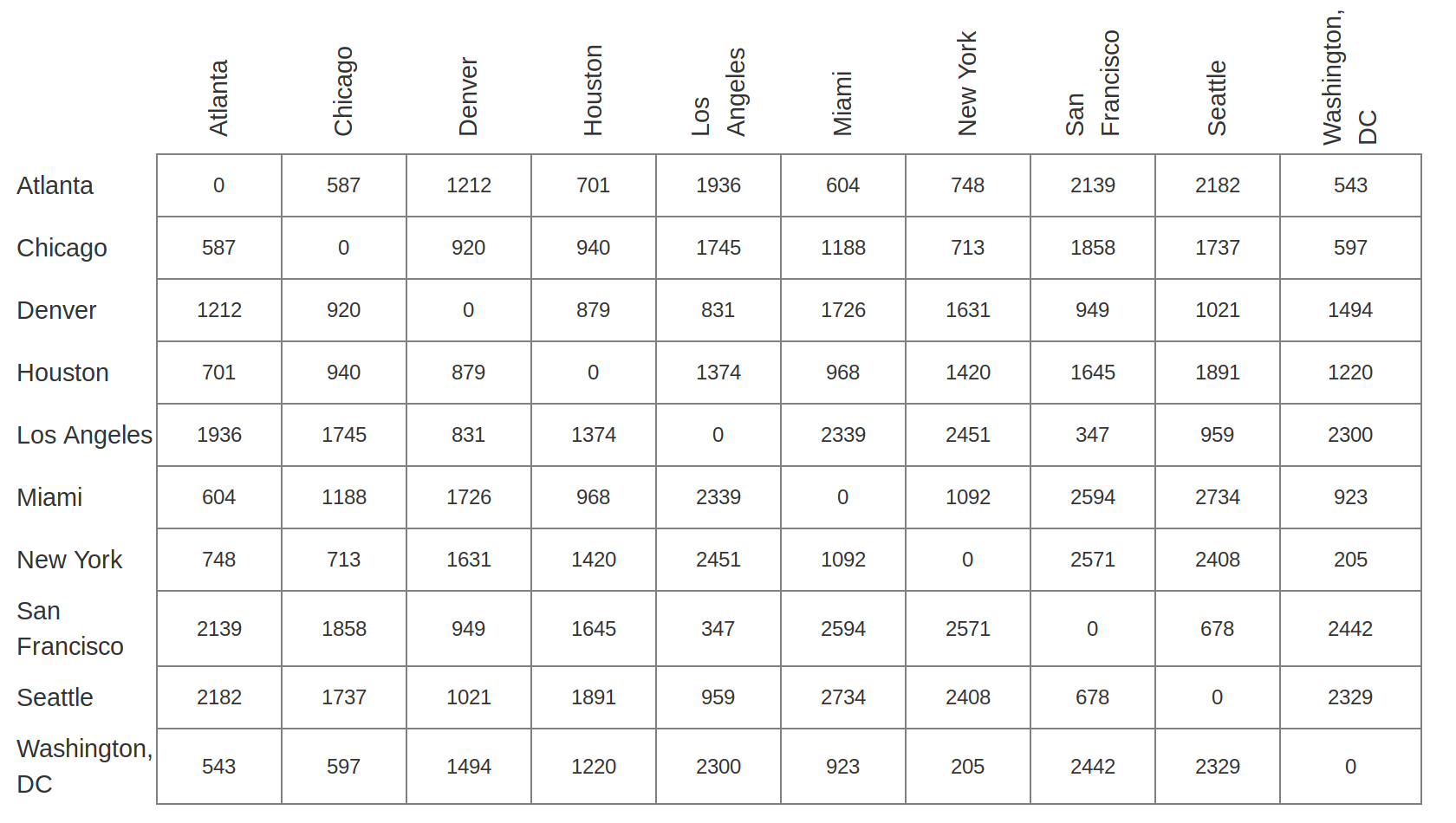
In this example, given data on the distance between different cities, we want map out the cities by finding their locations in a 2-dimensional coordinate system.
Below is an example of distance data that we may have available that will allow us to map a list of cities.
Let's load the data that we will be working with in this example.
city_data is an $n \times n$ numpy array where $n$ is the number of cities. city_data will store the table of distances between cities similar to the one above.
city_data = np.load('city_data.npy')
Before we start working with the data, we need to normalize the data by dividing by the largest element. This will allow us to more easily generate an initial guess for the location of each city.
city_data = city_data/np.max(city_data)
Below is a list of cities that we want to locate on a map.
city_names = [
    "Vancouver",
    "Portland",
    "New York",
    "Miami",
    "Mexico City",
    "Los Angeles",
    "Toronto",
    "Panama City",
    "Winnipeg",
    "Montreal",
    "San Francisco",
    "Calgary",
    "Chicago",
    "Halifax",
    "New Orleans",
    "Saskatoon",
    "Guatemala City",
    "Santa Fe",
    "Austin",
    "Edmonton",
    "Washington",
    "Phoenix",
    "Atlanta",
    "Seattle",
    "Denver"
  ]
Similar to the first example, the first step is to define the function that we need to minimize.
One way to formulate this problem is using the following loss function:
$$ loss({\bf X}) = \sum_i \sum_j (({\bf X}_i - {\bf X}_j)^T({\bf X}_i - {\bf X}_j) - D_{ij}^2)^2 $$
${\bf X}_i$ and ${\bf X}_j$ are the positions for cities $i$ and $j$. Each position ${\bf X}$ has two components, the $x$ and $y$ coordinates. These are the variables we want to find!
$({\bf X}_i - {\bf X}_j)^T({\bf X}_i - {\bf X}_j)$ is the squared-distance between cities $i$ and $j$, given the positions ${\bf X}_i$ and ${\bf X}_j$.
$D_{ij}$ is the known distance between cities $i$ and $j$. These are the given (known) variables provided in
city_data.
The loss function measures how much the actual location and the guess location differ. The optimization problem becomes:
$$ \min_{{\bf X}} loss({\bf X}) $$
Assume that the location of cities is stored as city_loc, a 1D numpy array of size $2n$, such that the x-coordinate of a given city is stored first followed by it's y-coordinate.
I.e. $$ \text{city_loc} = \begin{bmatrix} X_1[0]\\ X_1[1]\\ \vdots \\ X_n[0]\\ X_n[1] \end{bmatrix} $$
For example, if we had the cities Los Angeles, San Francisco and Chicago with their locations $(0.2,0.1),(0.2,0.5),(0.6,0.7)$, respectively, then city_loc would be
$$
\text{city_loc} =
\begin{bmatrix}
0.2\\
0.1\\
0.2 \\
0.5\\
0.6\\
0.7
\end{bmatrix}
.
$$
Write the loss function defined above, with the following signature:
def loss(city_loc, city_data):
    # city_loc: Numpy array of length 2n containing the x- and y-coordinates of all the cities
    # city_data: 2D Numpy array of length nxn containing the table of distances between cities
    # totalLoss: Scalar with the output of the loss function for a given set of locations of cities
    return totalLoss
Before we move on, let's check that our loss function is correct.
Check the output of your function on the following inputs. The loss function should evaluate to 0.2691297854852331.
city_loc = np.array([0.2,0.1,0.2,0.5,0.6,0.7])
print(loss(city_loc,city_data[:3,:3]))
Now that we have the function that we want to minimize, we need to compute it's gradient to use steepest descent.
$$ \begin{align} \frac{\partial loss}{\partial X_k} =& \sum_i -4 ((X_i-X_k)^T(X_i-X_k) - D_{ik}^2) (X_i-X_k) \\+& \sum_j 4 ((X_k-X_j)^T(X_k-X_j) D_{kj}^2) (X_k-X_j) \end{align} $$
We will give you one way to evaluate the gradient below. After lecture, make sure you can write this function for yourself. It is important to know how to obtain gradient of functions.
def gradientLoss(city_loc, city_data):
    n = len(city_loc)
    grad = np.zeros(n)

    for k in range(n//2):
        for i in range(n//2):
            xik = city_loc[2*i:2*i+2] - city_loc[2*k:2*k+2]
            grad[2*k:2*k+2] += -4 * (np.dot(xik,xik) - city_data[i,k]**2) * xik

        for j in range(n//2):
            xkj = city_loc[2*k:2*k+2] - city_loc[2*j:2*j+2]
            grad[2*k:2*k+2] += 4 * (np.dot(xkj,xkj) - city_data[k,j]**2) * xkj
    return grad
Let's check that our gradient function is correct. Using the same input as we used in testing our loss function, the resulting gradient should be
[ 0.14328835 -0.27303188 1.05797149 1.01695016 -1.20125985 -0.74391827].
city_loc = np.array([0.2,0.1,0.2,0.5,0.6,0.7])
print(gradientLoss(city_loc, city_data[:3,:3]))
We should now have everything that we need to use steepest descent if we use a learning rate instead of a line search parameter.
Steepest descent using learning rate
Write a function to run steepest descent for this problem.
Store the solution after each iteration of steepest descent in a list called
city_loc_history. To make plotting easier, we will reshapecity_locwhen we store it so that it is of shape $n \times 2$ instead of $2n$.Store the loss function after each iteration in a list called
loss_history.Your algorithm should not exceed a given maximum number of iterations.
In addition, you should add a convergence stopping criteria. Here assume that the change in the loss function from one iteration to the other should be smaller than a given tolerance
tol.
def steepest_descent(city_loc, learning_rate, city_data, num_iterations, tol):
    # compute num_iterations of steepest_descent
    city_loc_history = [city_loc.reshape(-1,2)]
    loss_history = []

    for i in range(num_iterations):

        # write step of steepest descent here

        loss_history.append( ... )

        city_loc_history.append(city_loc.reshape(-1,2))

        if (check if tolerance is reached):
            break

    return city_loc_history, loss_history
Using your steepest_descent function, find the location of each city.
Use a random initial guess for the location of each of the cities and use the following parameters.
learning_rate = 0.005
num_iterations = 300
tol = 1e-8
We can use the np.dstack function to change the list of city locations into a numpy array.
We will have a 3D numpy array with dimensions $n \times 2 \times num\_iterations$.
city_loc_history = np.dstack(city_loc_history)
Now let's display the location of each of the cities.
Note, you can use plt.text to display the name of the city on the plot next to its location instead of using a legend. The following code snippet will plot the final location of the cities if we assume that we stored the result of steepest descent as city_loc_history.
num_cities = city_loc_history.shape[0]

for i in range(num_cities):
    plt.scatter(city_loc_history[i,0,-1], city_loc_history[i,1,-1])
    plt.text(city_loc_history[i,0,-1], city_loc_history[i,1,-1], city_names[i])
plt.show()
Does your plot make sense? Keep in mind that we aren't keeping track of orientation (we don't have a fixed point for the origin) so you may need to "rotate" or "invert" your plot (mentally) for it to make sense. Or if you want an extra challenge for after class, you can modify the optimization problem to include a fixed origin :-)
You can plot the history of the loss function, and observe the convergence of the optimization (you can also try with semilogy)
plt.plot(loss_history, label = 'loss')
plt.xlabel('iteration')
plt.legend()
plt.show()
Let's also include how location of each of the cities changes throughout the optimization iterations. The following code snippet assumes that the output for steepest descent is stored in city_loc_history and is a numpy array of shape $n \times 2 \times num\_iterations$
num_cities = city_loc_history.shape[0]

for i in range(num_cities):
    plt.plot(city_loc_history[i,0,:], city_loc_history[i,1,:])
    plt.text(city_loc_history[i,0,-1], city_loc_history[i,1,-1], city_names[i])
plt.show()
The plot looks too cluttered, right? Repeat the same experiment but use a smaller number of cities. But don't forget to normalize the smaller data set. Use 10 cities for this smaller experiment.
Let's see how the loss changes after each iteration. Plot the loss_history variable.
plt.plot(loss_hist_2, label = 'loss')
plt.xlabel('iteration')
plt.legend()
plt.show()
Repeat the same experiment but try different values for the learning rate. What happens when we decrease the learning rate? Do we need more iterations? What happens when we increase the learning rate? Do we need more or less iterations?
Steepest descent with golden-section search
Now, let's use golden-section search again for computing the line search parameter instead of a learning rate.
Wrap the function that we are minimzing so that $\alpha$ is a parameter.
def objective_1d(alpha, city_loc, city_data):
    return loss(city_loc - alpha * gradientLoss(city_loc,city_data), city_data)
Rewrite your steepest descent function so that it uses scipy.optimize.golden.
Use your new function for steepest descent with line search to find the location of the cities and plot the result. You can use the code snippets for plotting that we provided above.
num_iterations = 300
tol = 1e-8

city_hist3, loss_hist3 = sd_line(city_loc2, city_data2, num_iterations, tol)
city_hist3 = np.dstack(city_hist3)

num_cities = city_hist3.shape[0]

for i in range(num_cities):
    plt.plot(city_hist3[i,0,:], city_hist3[i,1,:])
    plt.text(city_hist3[i,0,-1], city_hist3[i,1,-1], city_names[i])
plt.show()
What do you notice about how the solution evolves? Do you expect using a line search method that the solution will converge faster or slower? Will using a line search method increase the cost per iteration of steepest descent?
Plot the loss function at each iteration to see if it converges in fewer number of iterations.
plt.semilogy(loss_hist3, label = 'loss')
plt.xlabel('iteration')
plt.legend()
plt.show()
Using scipy function
We can now compare the functions you defined above with the minimize function from scipy
import scipy.optimize as sopt

num_cities = 6
tol = 1e-5

city_data_small = city_data[:num_cities,:num_cities]/np.max(city_data[:num_cities,:num_cities])
x0 = np.random.rand(2*city_data_small.shape[0])
# Providing only the function to the optimization algorithm
# Note that it takes a lot more function evaluations for the optimization, since
# gradient and Hessians are approximated in the backend
res1 = sopt.minimize(loss, x0, args=(city_data_small), tol=tol )
xopt1 = res1.x.reshape(num_cities,2)
print(xopt1)
print('Optimized loss value is ', res1.fun)
print('converged in', res1.nit, 'iteration with', res1.nfev, 'function evaluations' )
# Providing function and gradient to the optimization algorithm
# Note that the number of function evaluations are reduced, since only Hessian are now approximated
res2 = sopt.minimize(loss, x0, args=(city_data_small) , jac=gradientLoss, tol = tol )
xopt2 = res2.x.reshape(num_cities,2)
print(xopt2)
print('Optimized loss value is ', res2.fun)
print('converged in', res2.nit, 'iteration with', res2.nfev, 'function evaluations' )
xhist,loss_hist = sd_line(x0, city_data_6_cities, 400, tol)
xopt3 = xhist[-1]
print(xopt3)
print('Optimized loss value is ', loss_hist[-1])
print('convergend in ', len(loss_hist),'iterations')
xhist,loss_hist = steepest_descent(x0, 0.01,  city_data_6_cities, 400, tol)
xopt3 = xhist[-1]
print(xopt3)
print('Optimized loss value is ', loss_hist[-1])
print('convergend in ', len(loss_hist),'iterations')
num_cities = 6
for i in range(num_cities):
    plt.scatter(xopt1[i,0], xopt1[i,1])
    plt.text(xopt1[i,0], xopt1[i,1], city_names[i])
plt.show()
num_cities = 6
for i in range(num_cities):
    plt.scatter(xopt3[i,0], xopt3[i,1])
    plt.text(xopt3[i,0], xopt3[i,1], city_names[i])
plt.show()