lab_btree Belligerent BTrees
- Sunday, October 29 at 11:59 PM 10/29 @ 11:59 PM
Assignment Description
In this lab you’ll learn about BTrees and how they can be used to implement the dictionary ADT. Specifically you’ll learn about the algorithms involved in finding and inserting into a BTree. In addition to the algorithms, you’ll see why BTrees are a useful structure, and a potentially good alternative to self-balancing binary search trees.
The following serves primarily as a motivation for why BTrees are a useful structure. It’s not strictly necessary for completing the lab but it is nonetheless important. You will also be able see the potential advantages yourself when you chart the real-world speed difference between your BTree and a self-balancing binary search tree at the end of the lab.
Let us briefly venture away from the high-level land of CS 225 and talk about hardware and the real world. We will make a lot of simplifying assumptions and do a lot of hand-waving here since this isn’t the focus of this class. For a more formal treatment I will refer you to the nearest architecture class.
All computation for us is done by some sort of processor we will call the central processing unit (CPU). Modern CPUs can do several billion basic instructions (e.g. arithmetic operations on two values, moving small pieces of data around, &c.) every second. CPUs are cool! However, there’s a limitation: the CPU can only work on bits of data that are extremely close to it. These values are stored in “registers” — which are relatively simple circuits that can hold a fixed number of bits. The size of the normal registers on your computer is determined by the memory address size of your computer; i.e. if you have a “32-bit” machine, your memory addresses are 32 bits in size, and hence the registers on your computer can hold 32 bits. Similarly for “64-bit” machines, which are pretty much ubiquitous. The AMD64/x86-64 architecture (the predominant architecture for non-mobile computers at the moment) has 14 general purpose registers. That’s only 112 bytes. So the CPU can only “immediately” access around a hundred bytes of data. How does the CPU get access to more data? It has to load it into registers.
This is where the random access memory (RAM), or main memory, on your computer comes into play. The main memory on your computer can be pretty large compared to the paltry 112 bytes your CPU has access to. It’s not unusual for a regular laptop to have four or more gigabytes (~ $$4 \times 10^9$$ bytes) in its main memory. That’s a lot of bytes! However, there’s a catch. The CPU can access its registers immediately, but main memory is a lot “farther” away in circuit-land; it’s not an immediate operation to load something from main memory. We’ll say that it takes one clock cycle (remember that the CPU is doing several billion of these every second) to access a value from a register. To access something from main memory takes approximately 800 cycles (about 100 nanoseconds). Unfortunately this means that our CPU, if it wants something from main memory, is left twiddling its thumbs for 800 cycles until it can continue doing its computation.
Modern computers usually have a “level” of storage in between registers and main memory. It is closer to the CPU in terms of access time, but is significantly smaller than main memory. This region is called the “cache”, and it exists precisely because main memory is so slow compared to registers. While a load from main memory can take 800 CPU cycles, a load from the closest cache probably only takes about 4. The idea with the cache is to keep parts of main memory which are frequently used (or are likely to be used soon) close to the CPU so that it doesn’t have to go all the way to main memory. Caching is a very important part of modern computer architecture and it has a lot of real-world implications, some of which you’ll see later in this lab.
RAM and caches aren’t the end of the data storage story. After all, how does something get into RAM in the first place? It has to be loaded.
Before it can be loaded into RAM or registers, your data (programs, text, media, &c.) needs to be able to live somewhere persistently, i.e. not disappear when you turn off your computer. Neither RAM nor registers retain their data when the power gets turned off. There are two main forms of persistent storage in use today: hard disk drives (HDDs) and solid state drives (SSDs). The former use spinning magnetic disks, the latter uses billions of fancy circuits. Typical hard disk drives have access times of around 10 milliseconds ($$1 \times 10^7$$ nanoseconds), solid state drives around .1ms ($$1 \times 10^5$$ nanoseconds). Note the difference in order of magnitude between accessing something from RAM and accessing something from a HDD. (HDDs are still the kings of storage capacity; multi-terabyte (~$$10^{12}$$ bytes) HDDs aren’t uncommon.)
You should start to notice a pattern here: as we increase the amount of available storage there is a proportional increase in the amount of time it takes to get data to the CPU.
What’s even larger than a few terabytes on a HDD? How about your personal files somewhere in “the cloud”, i.e. on the internet? The space available with the internet is seemingly infinite, but it can be pretty slow too (just think about how long it takes to download a few dozen gigabytes over your typical internet connection compared to copying a few gigabytes from one part of a hard drive to another).
The Failings of Balanced BSTs
Suppose we have some obscenely large dictionary implemented as a balanced binary search tree. For example, suppose we want to store the US Census records in an AVL tree. There are approximately 317,814,000 people in the US according to the Census Bureau. Let’s say that each person has a unique entry in our AVL tree. On average, the height of an AVL tree is $$\log_2(n)$$, so for our record, we have a tree of height $$\log_2(317,814,000)$$; roughly 28. Doesn’t sound so bad right? 28 seems like a totally reasonable number. Well, until you consider how much data is probably in this tree. Suppose that for each of these keys we store a modest 512 bytes of data in the tree. That means that there’s approximately 163 GB of data associated with this tree. Yikes! That probably isn’t going to fit in the main memory of our computer. So what do we do instead? Well, we use the next largest thing in the storage hierarchy: a hard disk.
To see why the BST becomes a horrible choice when our data is on disk, let’s use a small on-disk AVL tree as an example:
Remember, none of these nodes are accessible to the CPU immediately; they all live on the hard disk. That means in the execution of our program, we have to fetch a node from the disk before the CPU can do anything with it. Earlier we said that each hard drive disk seek takes approximately 10ms, so suppose that we do a find operation, searching for 200 in the above tree. How much time do we spend just loading nodes from disk during that operation? Well, first we have to load the node 10, then 110, then 200. So in total that’s 30ms spent on loading nodes. Doesn’t seem so bad, but then you realize that our friend the CPU is crazy fast. 90ms is $$9 \times 10^7$$ nanoseconds. Our CPU can do about 8 instructions every nanosecond, which means that it could have done almost $$10^8$$ instructions in the time we spent loading those nodes! That’s a lot of wasted instructions. It gets considerably worse when we remember our large census AVL tree has a height of around 28.
BTrees to the Rescue
First, a quick definition. The (Knuth) order of a BTree is defined as the number of children each node can potentially have. You can also think of a BTree’s order as being one plus the maximum number of elements each node can have.
BTrees, unlike BSTs, store multiple keys (determined by the order of the tree) in each node, which limits the overall height of the tree. The nature of hard drives allows us to load a chunk of data all at once. Now when we are doing our search on the tree, each time we load a node we get a whole bunch of keys instead of just one. Once the nodes are in memory, the remaining time to process the entire node is negligible compared to the time it took to load them from disk (remember the orders of magnitude of difference between HDD access times and main memory access times).
Now let’s return to the example of the US Census data. We determined that the AVL tree for the data has a height around 28, which translates to a worst case of 28 disk accesses or 280ms of time “wasted” loading from disk. What if we used a BTree instead? Suppose that our BTree stores 64 keys in each node; this means that on each disk seek we will get 64 keys instead of just 1 with the AVL tree. A best case for the height of this BTree would be $$\log_{64}(317,814,000)$$; roughly 5. For this tree that means, in the worst case, we would have to load about 5 nodes from disk, meaning that we waste 50ms or so doing disk reads. Quite an improvement over 280ms!
As it turns out, the same logic can be applied to BTrees that live entirely in main memory. Just as RAM access time is significantly lower than HDD access time, cache access time is significantly lower than RAM access time. The same exact thing happens, except for instead of “wasting” time loading from disk, the CPU wastes time loading each node from main memory (remember it takes about 800 cycles to do that). RAM is similar to HDDs in that we can load a bunch of values at once into a faster medium. This means that we can get similar increases in performance by loading a bunch of keys from RAM into cache and then doing the processing to figure out where to go next in the tree. With extremely large data sets in memory, these small performance gains start to add up. In any situation where we can load a chunk of keys closer to the CPU in about the same amount of time it would take to load just one of them BTrees are potentially advantageous. This is why BTrees (or some variant of them) are used in file systems, databases, and even at Google (for massive in-memory dictionaries and sets). In this lab you’ll implement functions for an entirely in-memory BTree. You won’t have to worry about “loading” things into the cache — that’s all taken care of for you by the underlying architecture.
I highly suggest playing around with BTrees with this fun little app, as it really helps build your intuition for how the BTree algorithms work. Note that you can pause and step through the execution of the functions.
Checking Out The Code
You can get the code by updating your course repo. As usual, just run
svn up
from your cs225 directory. This will create a new folder in your working
directory called lab_btree.
The BTree Class and Friends
You’ll find the definition of the BTree class in btree.h. Just like
AVLTree, BTree is generic in that it can have arbitrary types for its keys
(assuming they can be compared) and values. There are two subclasses in
BTree: DataPair and BTreeNode. A DataPair is essentially just a key,
value pair which is useful since our BTree implements dictionary
functionality. The BTreeNode is a node in the BTree. It contains two
vectors: elements and children. elements is the data in the node,
children is pointers to the node’s child nodes. Note that DataPairs can be
compared with <, >, and == based entirely on their keys (the functions
are defined in the DataPair class).
Since BTreeNode uses vector pretty heavily, it would probably be a good
idea to keep a reference
open while working with them (in particular, vector’s insert and assign
functions will probably prove useful).
The Doxygen for the BTree class is here.
Note that due to the nature of the class, it will not be useful for you to
incrementally test things with provided test cases (except insertion_idx which
can be tested separately). Thus, you may write the functions in whatever order
makes sense to you and then debug them afterwards (using GDB is highly recommended).
A friend function of a class is defined outside that class’ scope but it has the right to access all private and protected members of the class. Even though the prototypes for friend functions appear in the class definition, friends are not member functions. You will not be required to create friend functions in this or any other tasks.
The insertion_idx Function
Doxygen for this function is here.
The elements of a BTreeNode are meant to be kept in sorted order so that they
can be searched with a binary search to quickly find the key in the node (if it
exists) or the proper child to explore. There’s a utility function in btree.h
called insertion_idx which serves this purpose. It is not specific to
BTree, rather it takes an arbitrary vector and arbitrary value and tries to
find the index in the vector the value can be inserted at such that the
vector will remain in sorted order. You should be able to safely use
operator<, operator>, and operator== inside this function when comparing
the parameter value to the elements in the vector. Thus, I should be able to do
something like this to insert 5 into the position that keeps sorted_vec
sorted:
/* sorted_vec is a sorted vector of ints */
size_t insert_idx = insertion_idx(sorted_vec, 5);
sorted_vec.insert(sorted_vec.begin() + insert_idx, 5);
You can test your function with provided test cases, or you can write your own testing functions for it somewhere.
The find Function
The Doxygen for this function is here.
Searching a BTree is very much like searching a BST. The main difference is
that instead of only having two possible children to explore, we have
order-many potential children. As with a BST, it is natural to write find
recursively. For a given level of the recursion, the steps are as follows.
First you must do a binary search on the elements (remember they should always
be stored in sorted order) using insertion_idx. If the key at insertion_idx
is the one we are looking for, we are done (since keys in the tree are unique)
and return, otherwise we didn’t find the key in the current node. If the
current node is a leaf node, then we’ve run out of nodes to explore and we are
also done. Otherwise, we need to call find recursively on the proper child
of the current node. This can be done using the return value of
insertion_idx.
Below is a few examples of find on a small, order 3 BTree.
The initial tree:
We search for 39. We start at the root, call insertion_idx, which should
return 2, since that’s the index in the root node that 39 could be inserted at
to maintain sorted order. Since this isn’t a valid index in the current node,
we know we need to explore a child. We also know that 2 is conveniently the index of
the child pointer (the bar) we want to explore.
We call insertion_idx on this node and find the key we are looking for.
Now let’s try finding something that isn’t in the tree, -2. We use
insertion_idx to find the place we would insert -2, which is index 0. This
is also the index of the child we want to explore.
When call insertion_idx on this node and find that the key is not in this
node. Since this node is also a leaf node, the key isn’t in the tree.
The split_child Function
The Doxygen for this function is here.
split_child is used as a part of the insertion process in a BTree to “fix”
the tree. When a node becomes “too full”, i.e. when its number of elements
becomes the tree’s order, we have to split the node into two nodes, and throw
out the median element into the parent node. The process should become more
clear with the below examples (combined with the insert examples). When
actually implementing this function you will probably want to use vector’s
assign function.
The insert Function
The Doxygen for this function is here.
You have to write the recursive helper function insert (the public one is
already written for you). Insertion into a BTree always happens at the leaf
nodes; inserting involves finding the proper leaf node (recursively) that the
key belongs in, and then “fixing” the tree on the way back up the recursive
calls.
As with find, first you should do a binary search on the current node being
explored. If the key we are trying to insert exists in the current node, then
there’s no more work to be done (don’t replace the value associated with the
already existing key).
Below is an example that illustrate the insertion/splitting process. Let’s start with 13.
We find the child we want to insert into in the same way as find. We have
to verify that the key isn’t in the current node and then recursively call
insert until we hit a leaf node to insert into.
We use insertion_idx at the leaf to find which spot the key belongs in.
Now let’s do an insert the requires a split; let’s insert 25.
Same process as with finding 25, we use insertion_idx to find the child to
recursively explore.
We insert 25 to the place it belongs in the leaf, and we are done at this
level of recursion. After the return (i.e. when we are back at the node
containing 8, 20) we check the size of the node we just inserted into. We see
that its size is equal to order, so we have to split it (using split_child).
First we find the median of the node we are splitting (element 25) put it at
the proper place in the 8, 20 node. We have to create a new node containing
everything to the right of 25 (including the child pointers to the right of
25). Similarly, the left node contains everything to left of 25. We have to
make sure to add the new right child pointer to the children of the 8, 20 node.
At this point we notice that the root has to be split.
The median of the current root (20) gets put into a new root node, and its two children are the 8 node and the 25 node.
Take note of the children indices that ended up in the two children nodes. 20 had index 1 in the original node. The child pointers that ended up in the left node had indices 0 and 1, the child pointers that ended up in the left node had indices 2 and 3. Note that for trees of odd order this ends up working out very nicely, since there’s only one choice of median. You have to be very careful though since this is not the case for even orders.
Testing Your Code
There are provided tests for the lab as per usual. There is also an executable
called test_btree, made by running:
make test_btree
If you run it with no parameters it will default to some basic tests with sequential and random integer data. It also can take parameters:
USAGE: test_btree ORDER N
Tests N inserts and N finds on a BTree<int, int> of order ORDER.
Additionally, note that BTreeNodes can be printed (see here).
E.g. if I’m in find I can do something like:
cout << *subroot << endl;
Committing Your Code
Commit your code the usual way:
svn ci -m "lab_btree submission"
Grading Information
The following files are used in grading:
btree.hbtree.cpp
All other files will not be used for grading.
Race Against std::map
The following isn’t really required to do the lab, but we think it’s an interesting way to see how your BTree is faster than the STL dictionary structure.
You must have matplotlib installed in order for the plots to work:
So you made this BTree, now how good is it really? Well, you can find out by
using the dict_racer executable. The usage is as follows:
USAGE: dict_racer ORDER N STEP RANDOM INSERTS FINDS
Runs a race between a BTree<int, int> of order ORDER against an
std::map<int, int> for N inserts / finds. Outputs CSVs into "results".
ORDER specifies the order of the BTree
N specifies the max number of insert / finds to do
STEP specifies the intervals to split N into. E.g. N = 10, STEP = 2 will make
points for 2 operations, 4 operations ... &c.
RANDOM specifies whether the data should be random or sequential.
INSERT specifies whether to benchmark the inserts.
FINDS specifies whether to benchmark the finds.
Results can be plotted with the simple python script generate_plot.py, e.g.
./generate_plot.py results/*.csv
For example, the following image was produced with the following commands on my laptop:
make dict_racer
./dict_racer 64 200000 1000 true true true
./generate_plot.py results/*.csv
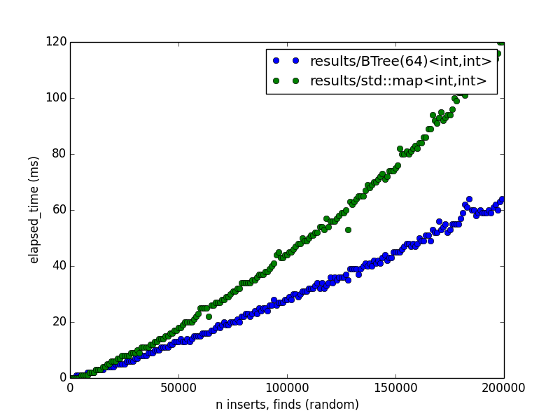
std::map in this case is implemented with a form of self-balancing binary
search tree called a red-black tree. As you can see, the difference in
performance widens as we increase $$n$$. I would guess that this is mostly
because the BTree keeps more of the data its processing in cache most of the
time, which is faster than loading each key, value from memory during a
traversal (which is what a binary search tree needs to do).
It’s worth experimenting with different orders, values for $$n$$, and step values. I wouldn’t recommend testing on EWS remotely as they’re shared machines and performance numbers are mostly meaningless. Also note that the Python script is very simple, so only keep CSVs around that have different values for order and step size, otherwise the plot will look pretty weird. Alternatively you can just remove the results directory each time.