Activity 5: First Steps with d3.js
Due: On git by Tuesday, Sept. 13, 2016 at 11:00am
Team: This is a solo assignment.
Grading: This assignment is the post-lecture activity for Experience 2,
worth 10 points. There is no partial credit.
Team: This is a solo assignment.
Grading: This assignment is the post-lecture activity for Experience 2, worth 10 points. There is no partial credit.
Initial Files
A new directory has been created on the git repository, which you should complete this assignment in. To merge this into your repository, navigate to your workbook directory using a command line and run the following commands:
git merge release/exp_activity5 master -m "merge"
Assignment Overview
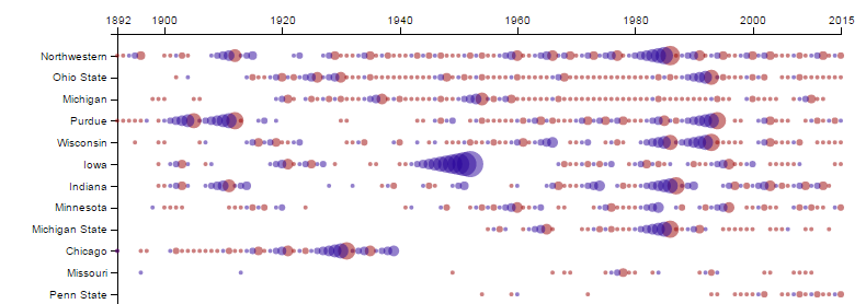
The goal of this assignment is to complete the key steps in creating a visualization. At the end of this assignment, you will have created a visualization similar to the following:
This assignment is broken up into two parts:
- Data Processing: You will complete compute.py to compute the current win streak of the Illini (used in the visualization as the radius of the circle).
- Visual Encoding: You will complete vis.js to visually encode the data you computed in the data processing step.
Part 1: Data Processing
In compute.py, add a new dictionary entry to each row called Streak.
This value should be the Illini win streak against the team from the preceding years.
For example, consider the 1953 Illinois vs. Michigan game, which is found in line 690 of illiniFootballScores_1892_2015.csv:
To find the Illini win streak coming into this game, you must find the game from the previous years and find the results of the games until the Illini lost or didn't play that team:
1951,3-Nov,vs.,Michigan,W,7,0,,,
1950,4-Nov,@,Michigan,W,7,0,,,
1949,29-Oct,vs.,Michigan,L,0,13,,,
Coming into the 1953 Illinois vs. Michigan game, the Illini were on a 3 game winning streak since the Illini won the game in 1952, 1951, and 1950 and lost the game in 1949.
The output for the 1953 Illinois vs. Michigan game should be the following in the JSON:
"Streak": 3
"Season": "1953",
"Opponent": "Michigan",
"IlliniScore": "19",
"OpponentScore": "3",
"Date": "7-Nov",
"Result": "W",
"Location": "vs.",
"Note1": "",
"Note2": "",
"Note3": "",
},
This can be completed by simply adding the code below once you have the streak calculated in a variable streak:
Part 1.5: Verify that the JSON is correct
Before starting with the visual encoding, ensure your JSON is correct. Open your JSON and verify that the 1953 Michigan game matches the data above. (The order of the entries in the dictionary will be different, but all the entries should be there.)
Only once you are certain your data is correct, continue to the visual encoding.
Part 2: Visual Encoding
Open vis.js (inside of your web directory) and jump down to Line 132, which starts the visual encodings:
.data(data)
.enter()
.append("circle")
To complete the visual encoding, you must define the cx,
cy, r, and fill attributes for
each circle. We have already defined two scales to help you with the
cx and cy. You can use the following code
(in bold) to correctly position the circles:
.data(data)
.enter()
.append("circle")
.attr("cx", function (d, i) {
return yearsScale( d["Season"] );
})
.attr("cy", function (d, i) {
return teamsScale( d["Opponent"] );
})
Continue with the code to define a r and fill
attribute. You can use the HSL Color Picker by Brandon Mathis
as a good way to find a good color for wins and losses.
Use your workbook to view your visualization. If you do not see any visualization, you can use the console in your web browser (Right Click, Inspect, and choose the Console tab).
Submission
This activity is submitted digitally via git. View detailed submission instructions here.