Activity 10: Simulation of a State Tree

Due: On git by Thursday, Oct. 27, 2016 at 11:00am
Team: This is a solo assignment; you should type all the code to your solution. However, feel free to get help from others/Google/etc.
Grading: This assignment is the mid-week activity for Experience 8, worth 10 points. There is no partial credit.

Introduction

In lecture, you learned a new two-player game with a very simple rule set:

• Each game starts with 10 marks
• Player 1 and Player 2 alternate turns:
  • Each turn, a player may pick up 1 or 2 marks
• The player who picks up the last mark wins

In lecture, you played several rounds of this game and, together, we developed a state space for this game. We decided that each state is described by two features: the current player's turn and the number of marks available.

From there, we developed a compact notation for this state space: p#-$, where # is the current player (either 1 or 2) and $ is the number of marks available.

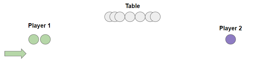
As an example, p1-7 notates that it is Player 1's turn and there are 7 marks left on the table. Visually, this implies that the game is at this state:

Part 1: Setup

The code that was finished in class has been provided as the starting code for this activity, in the exp_activity10 branch:

Part 2: Understanding the State Space Graph

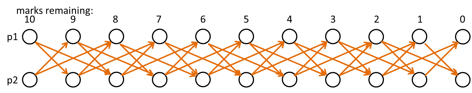
In the code provided, an exhaustive state space graph has been created. Each node is a valid game state and the collection of all nodes is every possible game state. Each edge is a valid move between states.

When the game begins at p1-10, Player 1 may pick up one or two marks. Therefore, p1-10 has edges to p2-9 and p2-8. Visually, this full graph is rendered below:

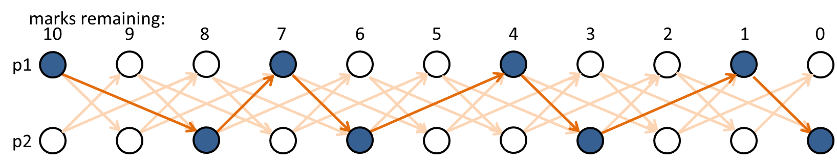
Every path through the graph is a valid game. One path, for example, is the following:

We can also represent this path through the state space graph visually:

Part 3: Simulating Games to Learn Edge

The goal of this activity is to have the machine learn the best edges to take in a game. To do this, we will simulate thousands of games and record which edges contributed to the win.

Similar to Activity 9, the provided code provided a path through the graph. Different from Activity 9, your responsibility is to update the edges on the graph along the path in the following way:

• Update every edge along the path by adding 1 to the weight edge attribute if the edge is an edge from the winning player to the losing player.
• Update every edge along the path by subtracting 1 to the weight edge attribute if the edge is an edge from the winning player to the losing player.

To complete this activity, program this logic in the updateEdgesBasedOnPath function found near the top of compute.py. The function takes in two arguments and does not need to return a value:

• G, a NetworkX graph of the state tree described in Part 2
• path, an array of node identifiers. For example:
  ["p1-10", "p2-8", "p1-7", "p2-6", "p1-4", "p2-3", "p1-1", "p2-0"]

Example:

Thinking back to the example in Part 2, the following path was given:

From this path, Player 1 won since Player 1 took the last mark. Therefore, all of the edges from Player 1 to Player 2 are updated by adding one to the weight and all edges from Player 2 to Player 1 are updated by subtracting one from the weight:

• p1-10 ➜ p2-8, add one to weight
• p2-8 ➜ p1-7, subtract one from weight
• p1-7 ➜ p2-6, add one to weight
• p2-6 ➜ p1-4, subtract one from weight
• p1-4 ➜ p2-3, add one to weight
• p2-3 ➜ p1-1, subtract one from weight
• p1-1 ➜ p2-0, add one to weight

Part 4: The Visualization

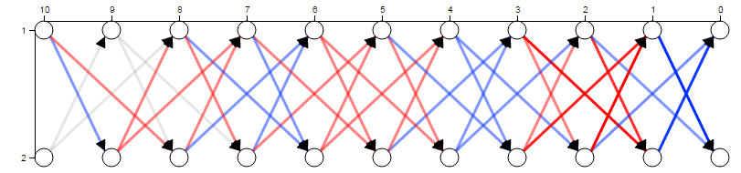
After you have completed the updateEdgesBasedOnPath function, running your Python will store your graph. A visualization has been provided that allows you to view the graph where the edges are visually encoded to show the weight stored in each edge attribute:

Submission

This activity is submitted digitally via git. View detailed submission instructions here.